Magic in R and Rust
2025-05-06
magic.RmdOverview of Magic implemented in R and Rust
(“Markov Affinity-based Graph Imputation of Cells” – van Dijk et al., 2018)
| Symbol | Size | Meaning |
|---|---|---|
| X | n × g | raw (or PCA-reduced) expression; rows = cells, cols = genes |
| d(i,j) | – | Euclidean (or cosine) distance between cell i and j in PCA space |
| σᵢ | – | local scale for cell i (distance to its k-th nearest neighbour) |
| A | n × n | symmetrised, locally scaled affinity (“heat”) matrix |
| D | n × n | diagonal degree matrix, Dii = ∑jAij |
| P = D⁻¹A | n × n | row-stochastic Markov transition matrix |
| t | – | diffusion time (walk length) |
| Ŷ | n × g | imputed expression after diffusion |
1 k-NN graph in latent space
Compute k nearest neighbours in the m-dimensional PCA space (typically k ≈ 30, m ≈ 100).
This is done by Seurat or related packages.
2 Adaptive Gaussian kernel
For each edge (i, j) in that graph set
$$ A_{ij} \;=\; \begin{cases} \displaystyle \exp\!\Bigl(-\frac{d(i,j)^2}{\sigma_i\,\sigma_j}\Bigr), & j\in\mathrm{kNN}(i),\\[6pt] 0, & \text{otherwise.} \end{cases} $$
Local bandwidths σᵢ make the kernel anisotropic so dense and sparse regions of the manifold are treated equally.
3 Markov normalisation
Now each row of P sums to 1 → one step of a random walk on the cell graph.
This is done in R:
4 Diffusion (raise to power t)
There are two equivalent views:
-
Spectral Diagonalise P = Ψ Λ Ψ⁻¹ with eigenvalues 1 = λ₀ > λ₁ ≥ λ₂ … Then
Small eigenmodes (high-frequency noise) decay as λₖᵗ.
Random-walk Entry (i,j) of Pᵗ is the probability that a random walk of length t starting at cell i ends in cell j.
5 Imputation by heat propagation
Apply the diffusion operator to every gene vector:
Each imputed expression value becomes a weighted average over the t-step neighbourhood, smoothing drop-outs while respecting manifold structure.
Relation to the continuous heat equation
On a smooth data manifold M, the generator L = I – P approximates the Laplace–Beltrami operator ΔM. Diffusion time t therefore controls how far one solves the heat-equation
MAGIC performs this on a graph and stops at a user-chosen t (often 2–6); too small → little denoising, too large → over-smoothing.
Blended MAGIC imputation
We have added an additional lever which controls the strength of the diffusion process.
Let
- be the original (cells × genes) expression matrix,
- the row-stochastic diffusion operator,
- the number of diffusion steps,
- the fully-diffused matrix,
- the blending weight.
We define the blended imputation
$$ X_{\rm imp}(\alpha) \;=\; (1 - \alpha)\,X \;+\; \alpha\,\widetilde X \;=\; (1 - \alpha)\,X \;+\; \alpha\,P^{\,t}\,X \;\in\mathbb{R}^{n\times g}. $$
Special cases
$$ \begin{aligned} \alpha = 0:\quad &X_{\rm imp}(0) = X,\\ \alpha = 1:\quad &X_{\rm imp}(1) = P^{t}X,\\ 0 < \alpha < 1:\quad &\text{Partial smoothing (convex blend of $X$ and $P^{t}X$).} \end{aligned} $$
How to run MAGIC in R/Rust
First we take some data, subset to the tumor cells that express modest levels of CD33.
suppressPackageStartupMessages({
  library(Seurat)
  library(scCustomize)
  library(rustytools)
  library(magrittr)
})


seu <- readRDS("~/Fred Hutch Cancer Center/Furlan_Lab - General/experiments/patient_marrows/annon/AML101/aml101.cds")
seu$sb <- seu$geno %in% "0" & seu$seurat_clusters %in% c("0", "1", "2", "3", "4", "11")
seu <- seu[,seu$sb]
seu <- NormalizeData(seu, verbose = F) %>% ScaleData(verbose = F) %>% FindVariableFeatures(verbose = F) %>% RunPCA(npcs = 100, verbose = F)
ElbowPlot(seu, ndims = 100)
seu <- FindNeighbors(seu, dims = 1:35, verbose = F) %>% FindClusters(verbose = F) %>% RunUMAP(dims = 1:35, n.epochs = 500, verbose = F)
DimPlot(seu)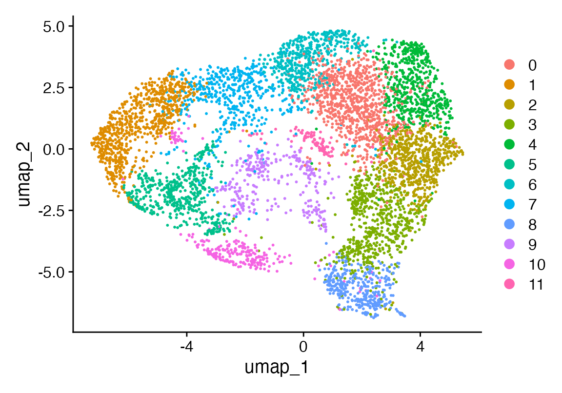
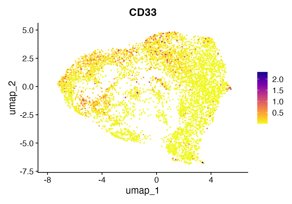
DefaultAssay(seu) <- "RNA"
FeaturePlot_scCustom(seu, "CD33")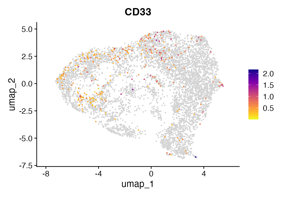
Now let’s see how they look after some magic.
seu <- seurat_magic(seu, alpha = 1)
DefaultAssay(seu) <- "MAGIC"
FeaturePlot_scCustom(seu, "CD33")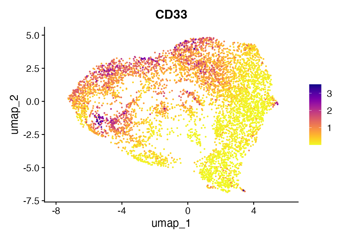
Changing parameters
An alpha of 1 might be too much. We can dial it back with an alpha of 0.3 and even further by dropping t to 2.
seu <- seurat_magic(seu, alpha = 0.3)

DefaultAssay(seu) <- "MAGIC"
FeaturePlot_scCustom(seu, "CD33")
seu <- seurat_magic(seu, alpha = 0.3, t = 2)

DefaultAssay(seu) <- "MAGIC"
FeaturePlot_scCustom(seu, "CD33")