How to deconvolute bulk RNAseq

Load a seurat object

This is an atlas of healthy bone marrow celltypes taken from:

Granja JM, Klemm S, McGinnis LM, Kathiria AS, Mezger A, Corces MR, Parks B, Gars E, Liedtke M, Zheng GXY, Chang HY, Majeti R, Greenleaf WJ. Single-cell multiomic analysis identifies regulatory programs in mixed-phenotype acute leukemia. Nat Biotechnol. 2019 Dec;37(12):1458-1465. doi: 10.1038/s41587-019-0332-7. Epub 2019 Dec 2. PMID: 31792411; PMCID: PMC7258684.

These data are not included in the viewmastR package.

suppressPackageStartupMessages({library(Seurat)
  library(viewmastR)
  library(magrittr)
  library(viridis)
  library(ggplot2)
  library(ComplexHeatmap)})

# Load single-cell data
sc_data <- readRDS(seurat_object_loc)
DimPlot(sc_data, group.by = "SFClassification", cols = sc_data@misc$colors)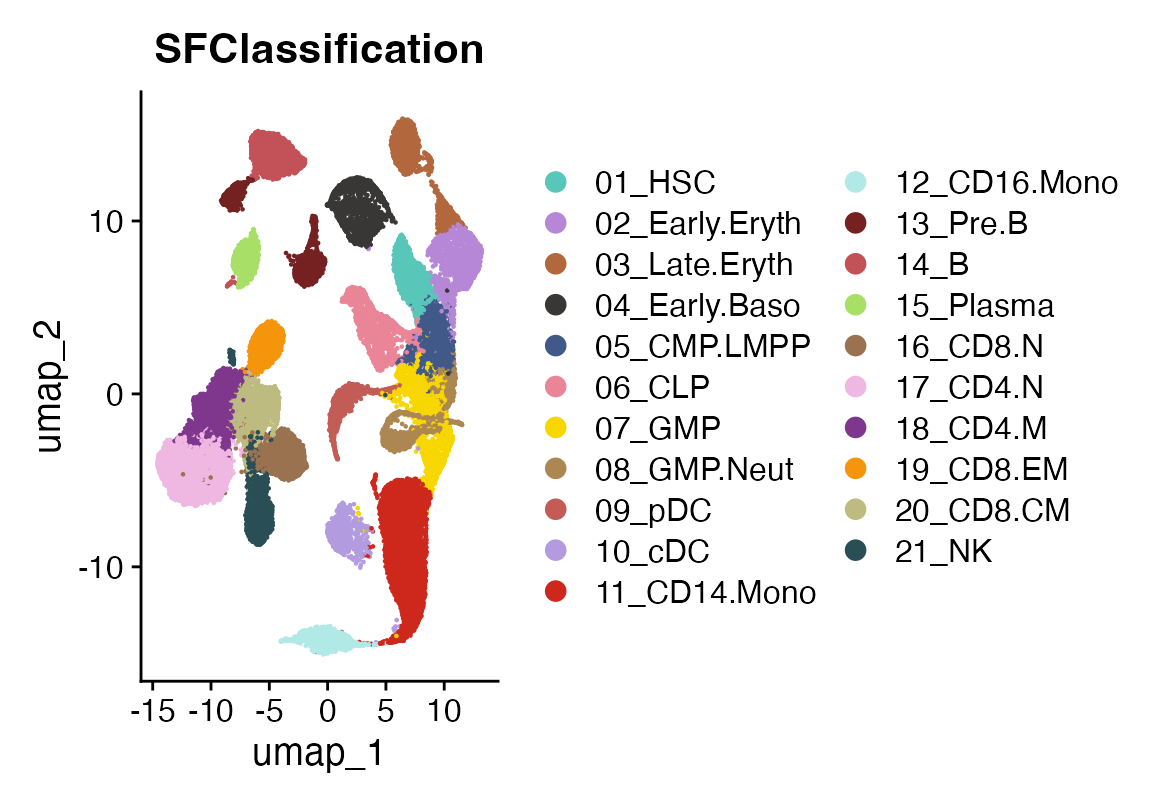

Now we pseudobulk the samples to get a matrix of “signatures”

# Extract normalized counts and cell type labels
counts <- GetAssayData(sc_data, layer = "data")  # log-normalized
cell_types <- sc_data$SFClassification

# Aggregate by cell type and create signatures
signatures <- sapply(unique(cell_types), function(ct) {
  cells <- which(cell_types == ct)
  rowMeans(expm1(counts[, cells]))  # expm1 reverses log1p normalization
})

Load bulk data

Next we load data released from the same publication that has bulk RNA seq from sorted populations of bone marrow cells. These data are included in the viewmastR package.

# Load bulk counts and gene lengths
bulk_counts <- system.file("extdata", "deconvolute", "GSE74246_RNAseq_All_Counts.txt", package = "viewmastR")
bulk_counts <- read.csv(bulk_counts, sep = "\t")
rn <- bulk_counts$X_TranscriptID
bulk_counts$X_TranscriptID<- NULL
bulk_counts <- as.matrix(bulk_counts)
rownames(bulk_counts) <- rn

gene_info <- read.table(system.file("extdata", "deconvolute", "geneWeights_withSymbol.tsv", package = "viewmastR"), header = TRUE)
rownames(gene_info) <- gene_info$symbol

Feature parity

Now we make sure the features are the same across all the data used for deconvolution. Check the dimensions to amake sure they match. We have 21 celltypes and 81 bulk samples. Here we find 18,879 features in common across all the inputs

# Ensure same genes
common_genes <- intersect(intersect(rownames(signatures), rownames(bulk_counts)), gene_info$symbol)
signatures <- signatures[common_genes, ]
bulk_counts <- bulk_counts[common_genes, ]

# Get gene lengths
gene_lengths <- gene_info[common_genes, "length"]
gene_weights <- gene_info[common_genes, "weight"]

dim(signatures)

## [1] 18879    21

dim(bulk_counts)

## [1] 18879    81

length(gene_lengths)

## [1] 18879

Deconvolute

You can read more on our implementation below, but here is a minimally working example using default parameters.

system.time(result_gd <- deconvolve_bulk(
  signatures = signatures,
  bulk_counts = bulk_counts,
  gene_lengths = gene_lengths,
  gene_weights = gene_weights, 
  max_iter = 3000
))

##    user  system elapsed 
##  61.057  14.026  74.937

system.time(result_em <- deconvolve_bulk(
  signatures = signatures,
  bulk_counts = bulk_counts,
  gene_lengths = gene_lengths,
  gene_weights = gene_weights, 
  max_iter = 3000,
  method = "em"
))

##    user  system elapsed 
##  14.968   2.100  16.779

Visualize

We will remove some of the bulk data that contains tumor cells or recombinant HSC for simplicity. We will also plot the Intercept as column annotation so one can get a sense of the degree of signal that is unaccounted for.

data <- as.matrix(result_gd$proportions_with_intercept)
data <- data[,!(grepl("LSC", colnames(data)) | grepl("rHSC", colnames(data)) | grepl("Blast", colnames(data)))]
cols <- pals::glasbey(13)
names(cols) <- unique(strsplit(colnames(data), "\\.") %>% sapply("[[", 2))
cola <- HeatmapAnnotation(bulk = strsplit(colnames(data), "\\.") %>% sapply("[[", 2), col = list(bulk=cols))
Heatmap(data[!rownames(data) %in% "Intercept",], top_annotation = cola, show_column_names = F, col = viridis(100), bottom_annotation = HeatmapAnnotation(Intercept = anno_points(data[rownames(data) %in% "Intercept",])), name = "GD Result")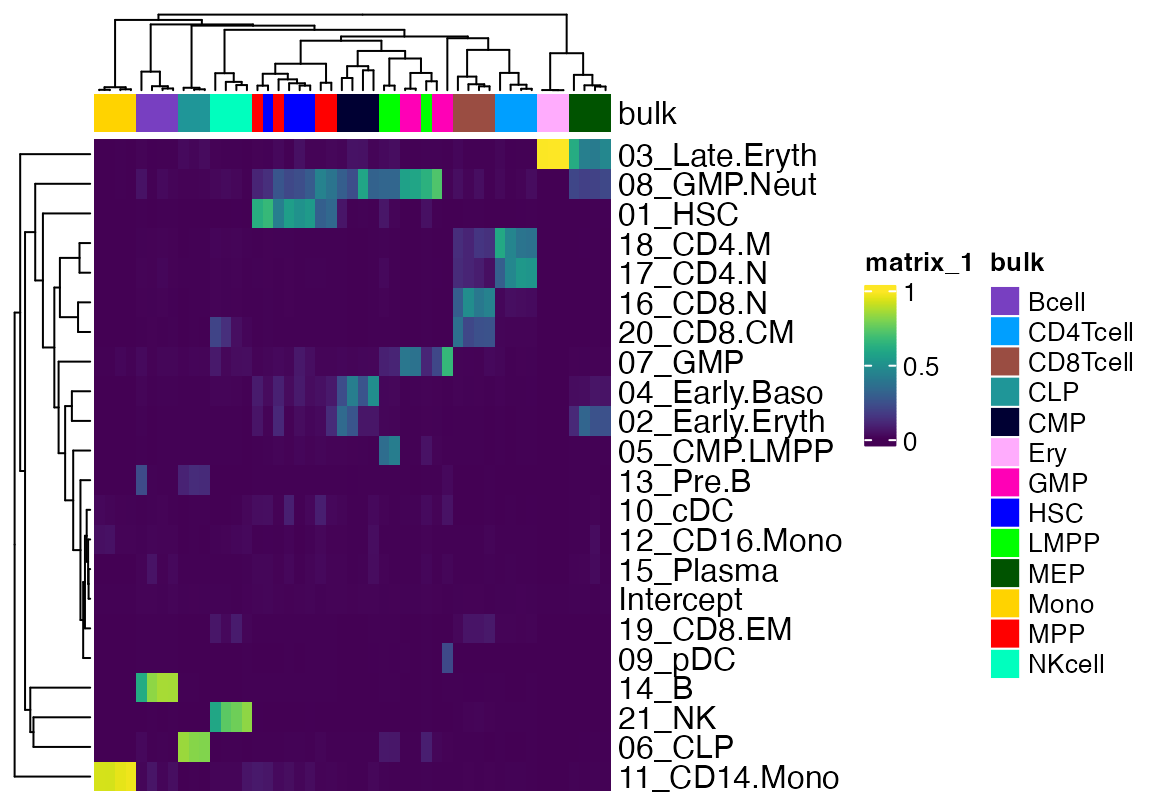

data <- as.matrix(result_em$proportions_with_intercept)
data <- data[,!(grepl("LSC", colnames(data)) | grepl("rHSC", colnames(data)) | grepl("Blast", colnames(data)))]
cols <- pals::glasbey(13)
names(cols) <- unique(strsplit(colnames(data), "\\.") %>% sapply("[[", 2))
cola <- HeatmapAnnotation(bulk = strsplit(colnames(data), "\\.") %>% sapply("[[", 2), col = list(bulk=cols))
Heatmap(data[!rownames(data) %in% "Intercept",], top_annotation = cola, show_column_names = F, col = viridis(100), bottom_annotation = HeatmapAnnotation(Intercept = anno_points(data[rownames(data) %in% "Intercept",])), name = "EM Result")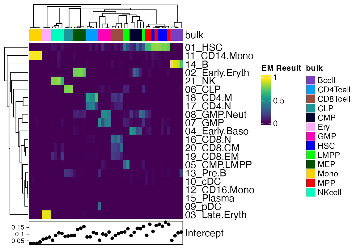

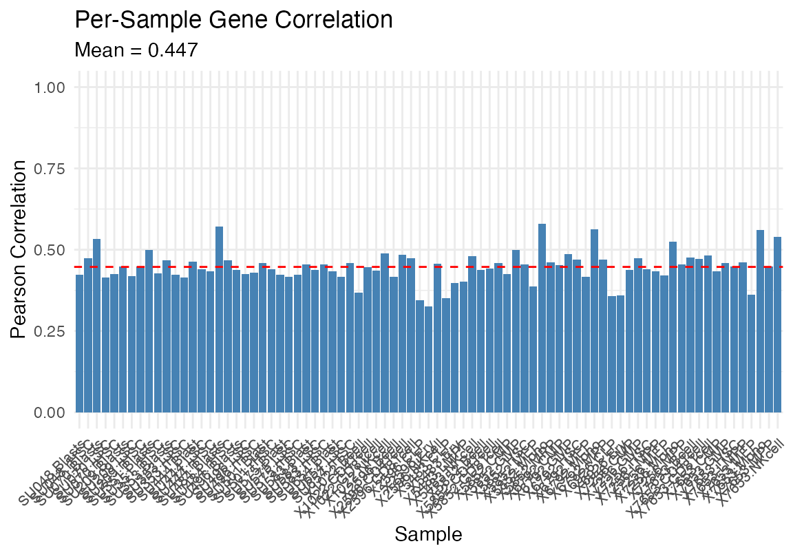
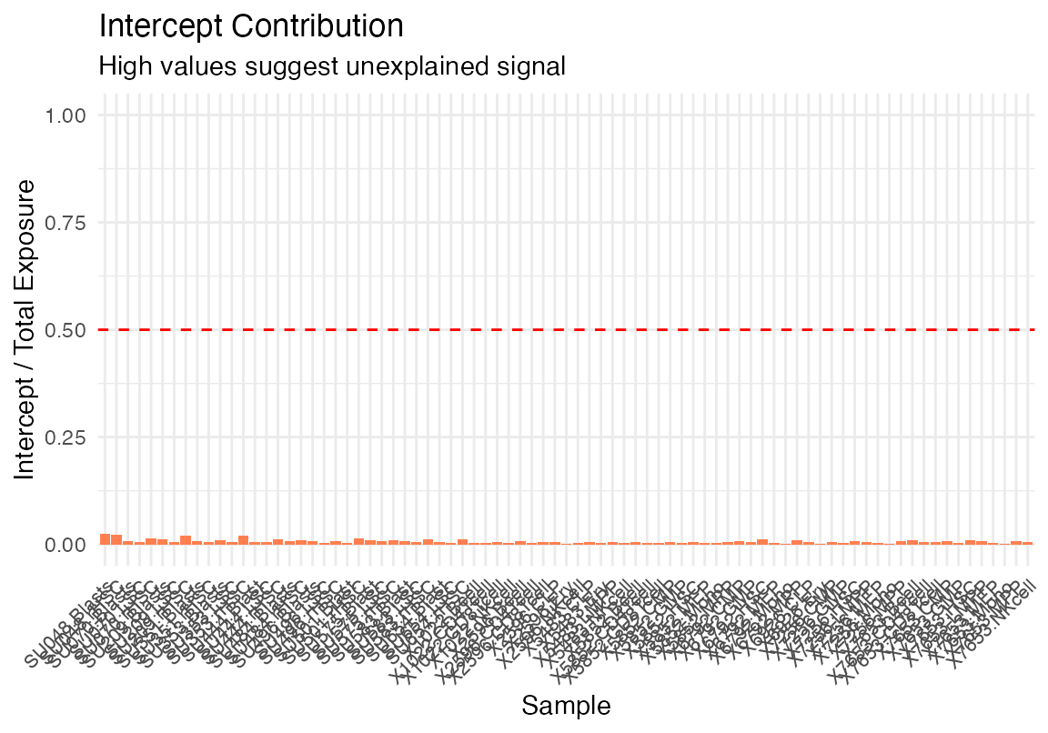
One can also use our build in plotting functions

plot_deconvolution(result_gd)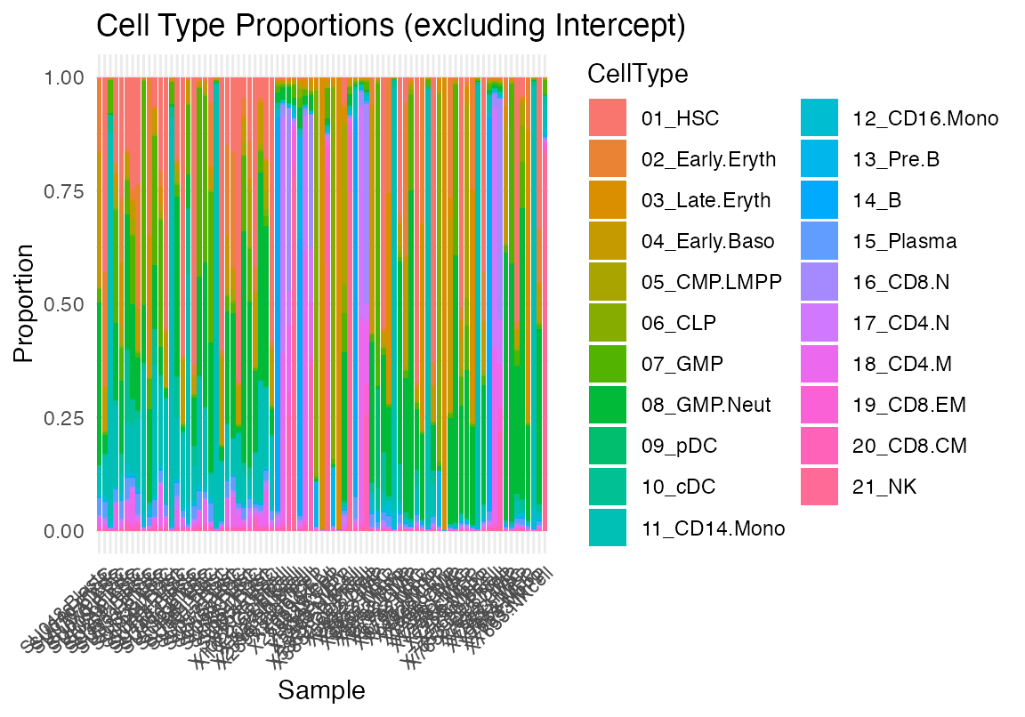

df <- data.frame(GradDescent=as.vector(as.matrix(result_gd$proportions_with_intercept)), ExpMax=as.vector(result_em$proportions_with_intercept), Celltype = rep(rownames(as.matrix(result_gd$proportions_with_intercept)), ncol(as.matrix(result_gd$proportions_with_intercept))), Sample = rep(strsplit(colnames(as.matrix(result_em$proportions_with_intercept)), "\\.") %>% sapply("[[", 2), each = nrow(as.matrix(result_em$proportions_with_intercept))))
g <- ggplot(df, aes(x=GradDescent, y=ExpMax, colour = Celltype))+geom_point()+scale_color_manual(values=c(sc_data@misc$colors, "Intercept"="black"))
plotly::ggplotly(g)

g <- ggplot(df, aes(x=GradDescent, y=ExpMax, colour = Sample))+geom_point()+scale_color_manual(values=pals::glasbey(17))
plotly::ggplotly(g)

cor(df$GradDescent, df$ExpMax)

## [1] 0.8536519

hex_plot <- function(result, bulk_counts){
  cor(as.vector(result$pred_counts[gene_weights>0,]), as.vector(bulk_counts[gene_weights>0,]))
  obs_flat <- as.vector(bulk_counts[gene_weights>0,])
  pred_flat <- as.vector(result$pred_counts[gene_weights>0,])
  # Remove zeros for log scale
  keep_idx <- obs_flat > 0 & pred_flat > 0
  fit_df <- data.frame(
    Observed = log1p(obs_flat[keep_idx]),
    Predicted = log1p(pred_flat[keep_idx])
  )
  rsq <- cor(fit_df$Observed, fit_df$Predicted)^2
ggplot(fit_df, aes(x=Observed, y=Predicted))+geom_hex(bins = 100)+scale_fill_viridis_c(trans = "log10")+ggtitle(rsq)
}



hex_plot(result_em, bulk_counts = bulk_counts)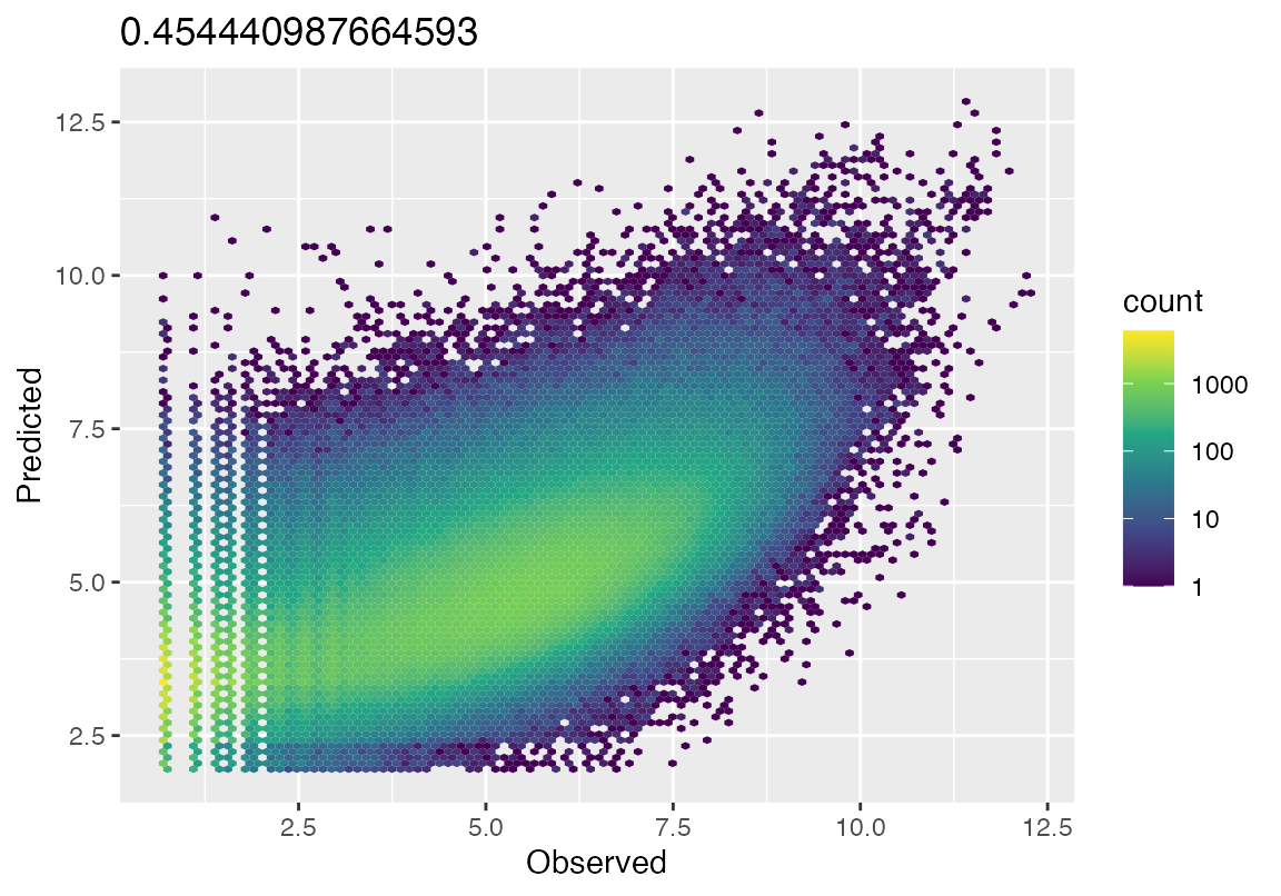

hex_plot(result_gd, bulk_counts = bulk_counts)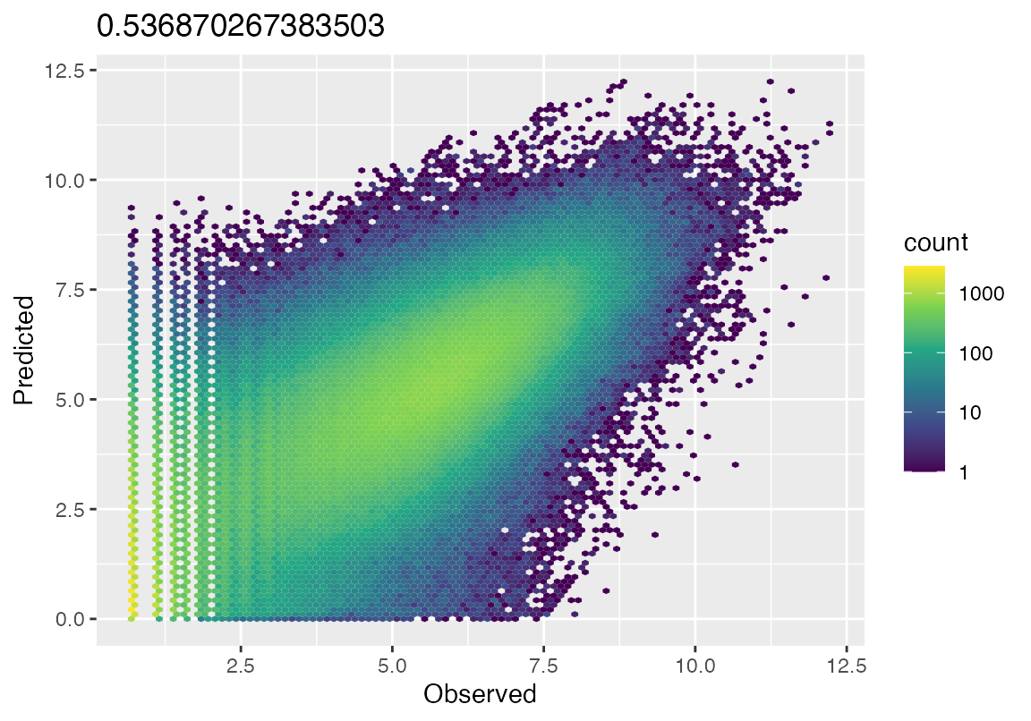

library(MuSiC)
library(SingleCellExperiment)
sce <- SingleCellExperiment(list(counts = sc_data@assays$RNA@counts), colData = DataFrame(sc_data@meta.data), rowData=DataFrame(symbol=rownames(sc_data)))

sce$sample <- "sample"

prop <- music_prop(bulk_counts, sce, markers = NULL, clusters = "SFClassification", samples = "orig.ident")

data <- as.matrix(t(prop$Est.prop.weighted))
data <- data[,!(grepl("LSC", colnames(data)) | grepl("rHSC", colnames(data)) | grepl("Blast", colnames(data)))]
cols <- pals::glasbey(13)
names(cols) <- unique(strsplit(colnames(data), "\\.") %>% sapply("[[", 2))
cola <- HeatmapAnnotation(bulk = strsplit(colnames(data), "\\.") %>% sapply("[[", 2), col = list(bulk=cols))
Heatmap(data, top_annotation = cola, show_column_names = F, col = viridis(100), name = "MuSiC Result")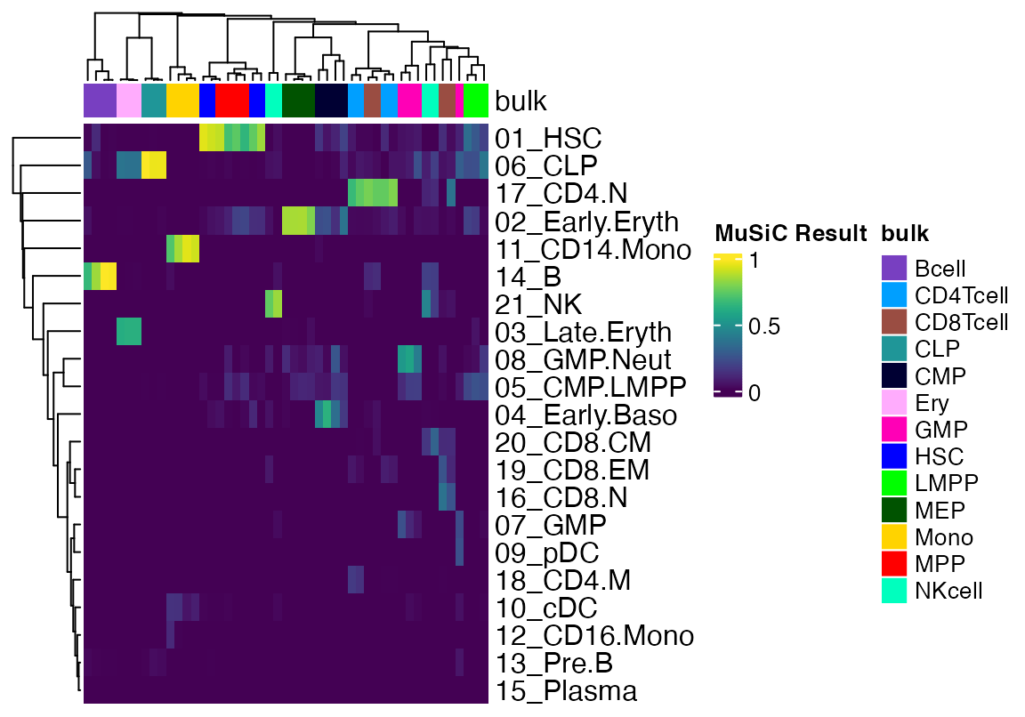

df <- data.frame(MuSiC=as.vector(as.matrix(t(prop$Est.prop.weighted))), ExpMax=as.vector(result_em$proportions), Celltype = rep(rownames(as.matrix(result_em$proportions)), ncol(as.matrix(result_em$proportions))), Sample = rep(strsplit(colnames(as.matrix(result_em$proportions)), "\\.") %>% sapply("[[", 2), each = nrow(as.matrix(result_em$proportions))))

g <- ggplot(df, aes(x=MuSiC, y=ExpMax, colour = Celltype))+geom_point()+scale_color_manual(values=c(sc_data@misc$colors, "Intercept"="black"))
plotly::ggplotly(g)

g <- ggplot(df, aes(x=MuSiC, y=ExpMax, colour = Sample))+geom_point()+scale_color_manual(values=pals::glasbey(17))
plotly::ggplotly(g)

cor(df$MuSiC, df$ExpMax)

## [1] 0.8682881

df <- data.frame(MuSiC=as.vector(as.matrix(t(prop$Est.prop.weighted))), GD=as.vector(result_gd$proportions), Celltype = rep(rownames(as.matrix(result_gd$proportions)), ncol(as.matrix(result_gd$proportions))), Sample = rep(strsplit(colnames(as.matrix(result_em$proportions)), "\\.") %>% sapply("[[", 2), each = nrow(as.matrix(result_em$proportions))))
g <- ggplot(df, aes(x=MuSiC, y=GD, colour = Celltype))+geom_point()+scale_color_manual(values=c(sc_data@misc$colors, "Intercept"="black"))
plotly::ggplotly(g)

g <- ggplot(df, aes(x=MuSiC, y=GD, colour = Sample))+geom_point()+scale_color_manual(values=pals::glasbey(17))
plotly::ggplotly(g)

cor(df$MuSiC, df$GD)

## [1] 0.7459681

Mathematical Summary of Poisson regression with gradient descent

Inputs: Signatures S (G×C), bulk counts k (G×N), gene lengths L, weights w
Output: Exposures E (C×N) = cell type abundances

Model

Forward Pass

q = [S | 1/G] × [E; intercept]              # Molecules
ŷ[g,n] = q[g,n] × (L[g] / insert_size)     # Reads
k[g,n] ~ Poisson(ŷ[g,n])                    # Observed counts

Parameterization

E = exp(log_E),  intercept = exp(log_intercept)
log_E[c,n] ~ Normal(-5, 0.1)  # Init breaks symmetry

Loss Function

NLL = Σ w[g] × [k·log(k) - k - k·log(ŷ+ε) + ŷ]  # Poisson likelihood
L₁  = λ₁ × (NLL/100) × Σ E                      # Sparsity penalty
L₂  = λ₂ × (NLL/100) × Σ E²                     # Stability penalty
Loss = NLL + L₁ + L₂

Optimization

Two phases: 1. NULL: Freeze E≈0, optimize intercept only → baseline 2. Full: Re-init E, optimize all parameters with Adam (lr=0.01)

Convergence: Stop when Δloss/loss < 10⁻⁶ AND Δsparsity < 10⁻⁴

Output

Exposures:   E[c,n] = exp(log_E[c,n])           # Cell-equivalents
Proportions: P[c,n] = E[c,n] / Σ_c E[c,n]       # Fractions (sum to 1)
Quality:     intercept / (Σ E + intercept)       # <0.1 = good fit

Key Parameters

Parameter	Default	Range	Purpose
`l1_lambda`	0	0-10	Sparsity (1=moderate, 5=strong)
`l2_lambda`	0	0-10	Stability (prevents extreme values)
`learning_rate`	0.01	0.001-0.1	Optimization step size
`insert_size`	500	150-500	Fragment length correction

Recommendation: Start with defaults (no regularization). Add l1_lambda=0.5-2 only if too many cell types.

Properties

Non-negativity: Guaranteed by exp() transform
Scale: Set by signature normalization (Σ S[g,c] = 1)
Gene length correction: Essential for RNA-seq (longer genes → more reads)
Performance: 10-30 sec GPU, 1-5 min CPU (typical: 18k genes, 21 types, 81 samples)

Mathematical Summary of Expectation-Maximization for Deconvolution

Inputs: Signatures S (G×C), bulk counts k (G×N), gene lengths L, weights w
Output: Exposures E (C×N) = cell type abundances

Probabilistic Model

Generative Process

For each gene g in sample n:
  1. Each read comes from source j ∈ {cell types, noise}
     P(source=j) ∝ S[g,j] × E[j,n]
  
  2. Noise has uniform signature: S[g,noise] = 1/G
  
  3. Observed counts: k[g,n] ~ Poisson(ŷ[g,n])
     where ŷ[g,n] = Σ_j S[g,j] × E[j,n] × (L[g] / insert_size)

Hidden Variable

z[g,j,n] = # of reads from gene g, sample n, assigned to source j
           (unobserved, inferred by EM)

EM Algorithm

E-step: Compute Responsibilities

For each source j (cell type or noise):
  contribution[g,j,n] = S[g,j] × E[j,n]
  
  responsibility[g,j,n] = contribution[g,j,n] / Σ_j' contribution[g,j',n]
  
Interpretation: "What fraction of counts for gene g came from source j?"

M-step: Update Exposures

For each source j:
  E[j,n] = Σ_g w[g] × k[g,n] × responsibility[g,j,n]
  
Interpretation: "Total weighted counts assigned to source j"

Intercept[n] = E[noise,n]  # Learned automatically

Log-Likelihood (Monitoring)

ŷ = [S | 1/G] × [E; intercept] × (L / insert_size)
LL = Σ w[g] × [k·log(ŷ+ε) - ŷ - k·log(k) + k]

Guarantee: LL increases every iteration (or numerical precision)

Optimization

Single unified phase (no null model needed!)

Initialize: E[c,n] = total_counts[n] / C
            intercept[n] = 0.05 × total_counts[n]

Repeat:
  1. E-step: Compute responsibilities for all sources
  2. M-step: Update E and intercept simultaneously
  3. Check: |ΔLL| < tolerance

Convergence: Typically 100-400 iterations

With L1 regularization:

After M-step: E ← max(E - λ₁, 0)  # Soft-thresholding

Output

Exposures:   E[c,n]                              # Cell-equivalents
Intercept:   intercept[n]                        # Noise level
Proportions: P[c,n] = E[c,n] / Σ_c E[c,n]       # Fractions (sum to 1)
Quality:     intercept / (mean(E) + intercept)   # <0.1 = good fit

Key Parameters

Parameter	Default	Range	Purpose
`l1_lambda`	0	0-10	Sparsity via soft-thresholding
`tolerance`	10⁻⁶	10⁻⁸-10⁻⁴	Convergence criterion (ΔLL)
`insert_size`	500	150-500	Fragment length correction
`max_iterations`	1000	100-10000	Safety limit

Recommendation: Defaults work well. No learning rate tuning needed!

Properties

Non-negativity: Guaranteed by model structure (no transforms needed)
Monotonic improvement: Log-likelihood never decreases
No hyperparameters: Learning rate, momentum, warmup not needed
Natural intercept: Noise competes with signatures automatically
Scale: Set by total counts and signature normalization
Gene length correction: Essential for RNA-seq (longer genes → more reads)
Performance: 15-25 sec (typical: 18k genes, 21 types, 81 samples, 300 iters)

Comparison to Gradient Descent

Aspect	EM	Gradient Descent
Convergence	Guaranteed monotonic	Can oscillate/diverge
Hyperparameters	None (just tolerance)	Learning rate, warmup
Iterations	100-400	1000-3000
Null model	Not needed	Requires separate fit
Interpretation	Missing data framework	Optimization of loss
Speed	15-25 sec	20-30 sec
Stability	Very stable	Needs careful tuning

Intuition

EM treats deconvolution as:
“For each read, which cell type (or noise) generated it?”

E-step: Probabilistically assign reads to sources
M-step: Count up assignments to estimate abundances

This “soft assignment” framework is more natural than gradient-based optimization for count data, leading to stable convergence without tuning.

2025-10-13

Load a seurat object

Load bulk data

Feature parity

Deconvolute

Visualize

Mathematical Summary of Poisson regression with gradient descent

Model

Forward Pass

Parameterization

Loss Function

Optimization

Output

Key Parameters

Properties

Mathematical Summary of Expectation-Maximization for Deconvolution

Probabilistic Model

Generative Process

Hidden Variable

EM Algorithm

E-step: Compute Responsibilities

M-step: Update Exposures

Log-Likelihood (Monitoring)

Optimization

Output

Key Parameters

Properties

Comparison to Gradient Descent

Intuition