Implementing Scrublet in R
2024-02-02
ImplementationHassles.RmdInstallation of packages
Note that this notebook was run using Rstudio enabling both R and Python environments to be maintained throughout.
Installing scrubletR
You will need to have the devtools package installed…
devtools::install_github("furlan-lab/scrubletR")Loading reticulate
Not for the faint of heart… You can read about getting python working from within R [here] (https://rstudio.github.io/reticulate/). You can either activate your reticulate environment and use ‘pip install scrublet’ to install scrublet or try from R as below. I use conda (reluctantly) and could not get it to install from in R
library(reticulate)
py_config()
py_install("scrublet")
I had to do this in the terminal after creating a new conda environment called ‘reticulate’.
Regardless of how you do it, you can check that it is installed using this from R. If you are successful, you will get no output.
py_run_string("import scrublet")Failure will look something like this
py_run_string("import scrubletoops")Comparing Implementations
Ok with working R and python versions of Scrublet, let’s go over the differences. First let’s load data
Load data
suppressPackageStartupMessages({
  library(viewmastR)
  library(Seurat)
  library(scCustomize)
  library(Matrix)
  library(ggplot2)
})

if(grepl("^gizmo", Sys.info()["nodename"])){
  ROOT_DIR2<-"/fh/fast/furlan_s/grp/data/ddata/BM_data"
} else {
  ROOT_DIR2<-"/Users/sfurlan/Library/CloudStorage/OneDrive-SharedLibraries-FredHutchinsonCancerCenter/Furlan_Lab - General/experiments/patient_marrows/aggr/cds/indy"
}

#query dataset
seuP<-readRDS(file.path(ROOT_DIR2, "220831_WC1.RDS"))
DimPlot_scCustom(seuP, label = F)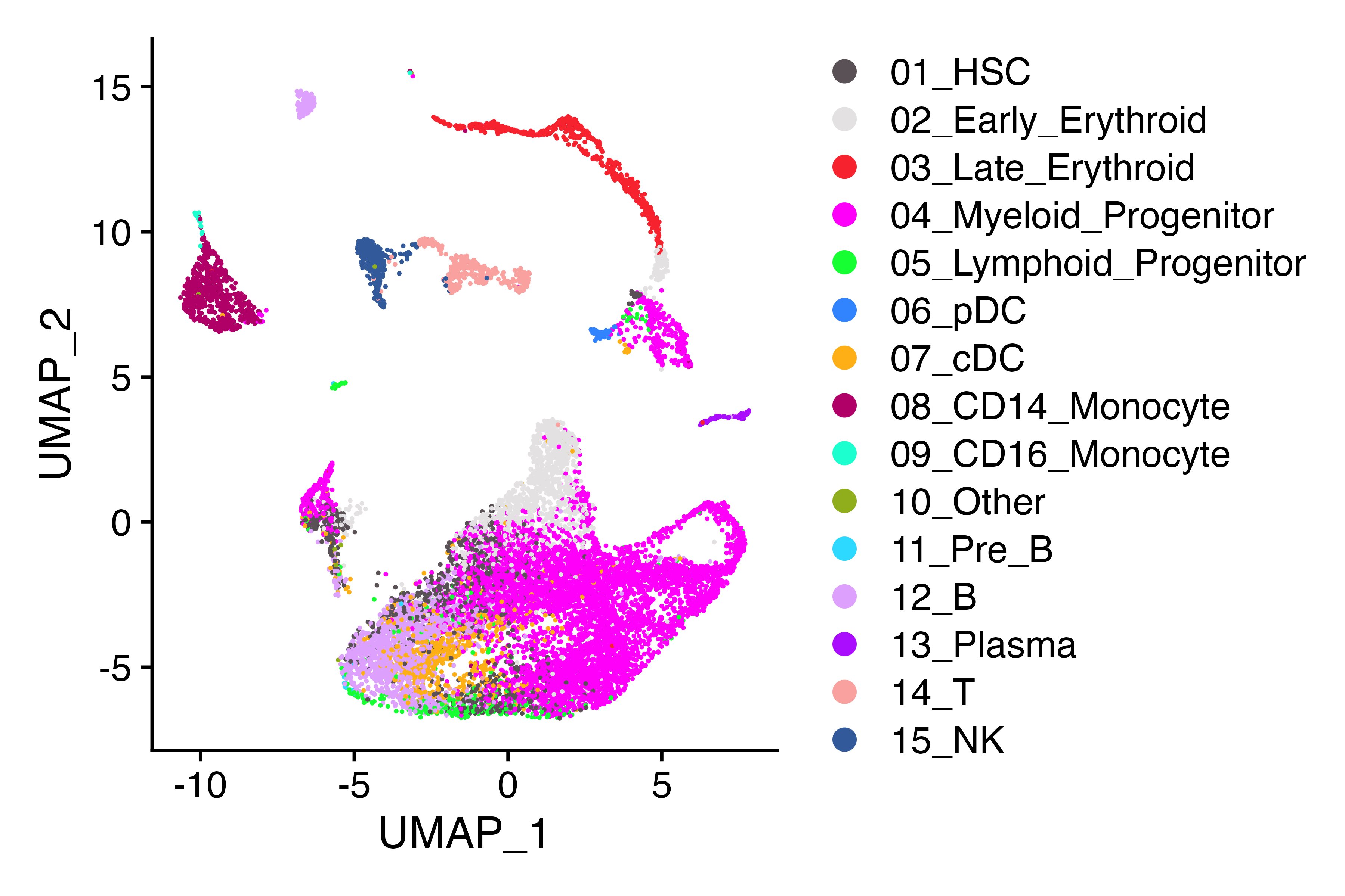
#counts_matrix<-t(seuP@assays$RNA@counts[,1:2000])
counts_matrix<-t(seuP@assays$RNA@counts)
First step
The first step in scrublet data processing is size factor normalization. Let’s see how the normalized counts compare across the two implementations. In the next block, I have run the scrublet pipeline through normalization and saved the counts in the R environment as “py_E_obs_norm”
import numpy as np
import scrublet as scr
scrub = scr.Scrublet(r.counts_matrix)

##set params
synthetic_doublet_umi_subsampling=1.0
use_approx_neighbors=True
distance_metric='euclidean'
get_doublet_neighbor_parents=False
min_counts=3
min_cells=3
min_gene_variability_pctl=85
log_transform=False
mean_center=True,
normalize_variance=True
n_prin_comps=30
svd_solver='arpack'
verbose=True
random_state = 0

#clear data in object
scrub._E_sim = None
scrub._E_obs_norm = None
scrub._E_sim_norm = None
scrub._gene_filter = np.arange(scrub._E_obs.shape[1])

#run normalize
scr.pipeline_normalize(scrub)

#capture size factor normalized counts
r.py_E_obs_norm = scrub._E_obs_norm.data
Run scrubletR size factor normalization
To see how the sets of counts compare, we can similarly run scrubletR normalization and correlate a sample (n=5000) of the log transformed counts using ggplot. Unsurprisingly they are not different.
#In R
#set params
synthetic_doublet_umi_subsampling = 1.0
use_approx_neighbors = TRUE
distance_metric = 'euclidean'
get_doublet_neighbor_parents = FALSE
min_counts = 3
min_cells = 3
min_gene_variability_pctl = 85
log_transform = FALSE
mean_center = T
normalize_variance = T
n_prin_comps = 30
verbose = TRUE


#instantiate object
scr<-ScrubletR$new(counts_matrix = counts_matrix)

scr$pipeline_normalize()

ix<-sample(1:length(scr$E_obs_norm@x), 5000)
ggplot(data.frame(x=log(scr$E_obs_norm@x[ix]), y = log(py_E_obs_norm[ix])), aes(x=x, y=y))+geom_point(size = 0.01)+xlab("scrubletR size-factor normalized counts")+ylab("scrublet (python) size-factor normalized counts")+theme_bw()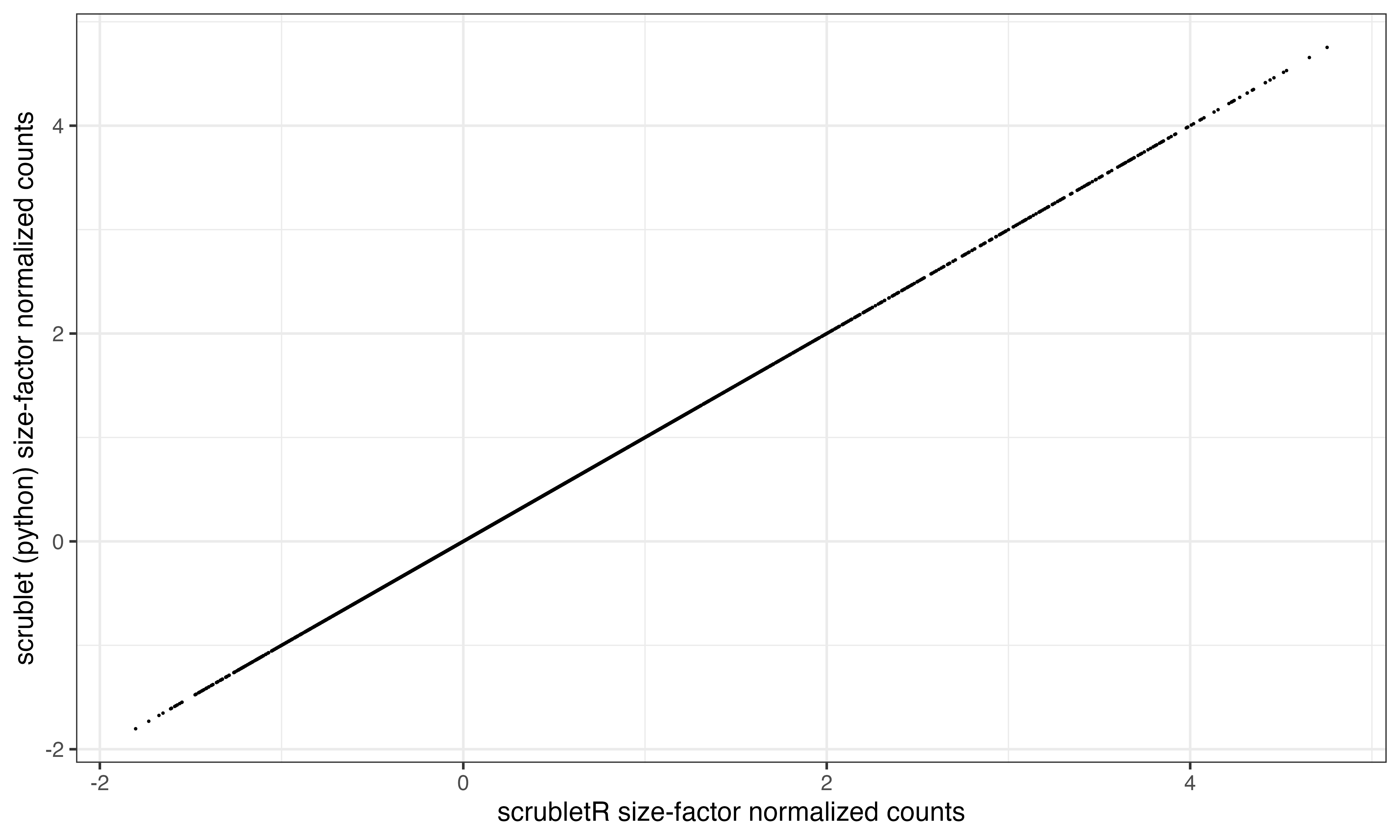
Second step
Next in the pipeline is to select a subset of features with the highest variable expression. The default is set to find the set of features that exhibit expression variance in the above the 85th percentile as measured using the v-statistic.
genefilter = scr.filter_genes(scrub._E_obs_norm,
                                        min_counts=min_counts,
                                        min_cells=min_cells,
                                        min_vscore_pctl=min_gene_variability_pctl, show_vscore_plot=False)
v_scores, CV_eff, CV_input, gene_ix, mu_gene, FF_gene, a, b = scr.get_vscores(scrub._E_obs_norm)
r.py_vscores = v_scores
min_vscore_pctl=min_gene_variability_pctl
ix2 = v_scores>0
v_scores = v_scores[ix2]
gene_ix = gene_ix[ix2]
mu_gene = mu_gene[ix2]
FF_gene = FF_gene[ix2]
min_vscore = np.percentile(v_scores, min_vscore_pctl)
final_ix = (((scrub._E_obs_norm[:,gene_ix] >= min_counts).sum(0).A.squeeze() >= min_cells) & (v_scores >= min_vscore))
Problem #1
V-scores are slightly different between R and python. The correlation is pretty good howewever and this likely won’t affect performance too much
vscores_result<-get_vscores(scr$E_obs_norm)
Vscores <- as.numeric(vscores_result$v_scores)


df<-data.frame(vscore_R=log(Vscores), vscore_py = log(py_vscores), indices_py=1:length(Vscores) %in% (py$gene_ix+1), indices_R=1:length(Vscores) %in% vscores_result$gene_ix)

df$selected_cat<-factor(with(df, 2*indices_py + indices_R + 1))
levels(df$selected_cat)<-c("neither", "both")


gene_ix <- vscores_result$gene_ix
mu_gene <- vscores_result$mu_gene
FF_gene <- vscores_result$FF_gene
a <- vscores_result$a
b <- vscores_result$b

ix2 <- Vscores > 0
Vscores <- Vscores[ix2]
gene_ix <- gene_ix[ix2]
mu_gene <- mu_gene[ix2]
FF_gene <- FF_gene[ix2]

min_vscore_pctl=min_gene_variability_pctl
min_vscore <- quantile(Vscores, prob = min_vscore_pctl / 100)

ix <- (colSums(scr$E_obs_norm[, gene_ix] >= min_counts) >= min_cells) & (Vscores >= min_vscore)

df$selected_R<-ix
df$selected_py<-py$final_ix
df$selected_cat<-factor(with(df, 2*selected_py + selected_R + 1))
levels(df$selected_cat)<-c("neither", "r_only", "py_only", "both")
ggplot(df, aes(x=vscore_R, y=vscore_py, color = selected_cat))+geom_point(size = 0.2)+theme_bw()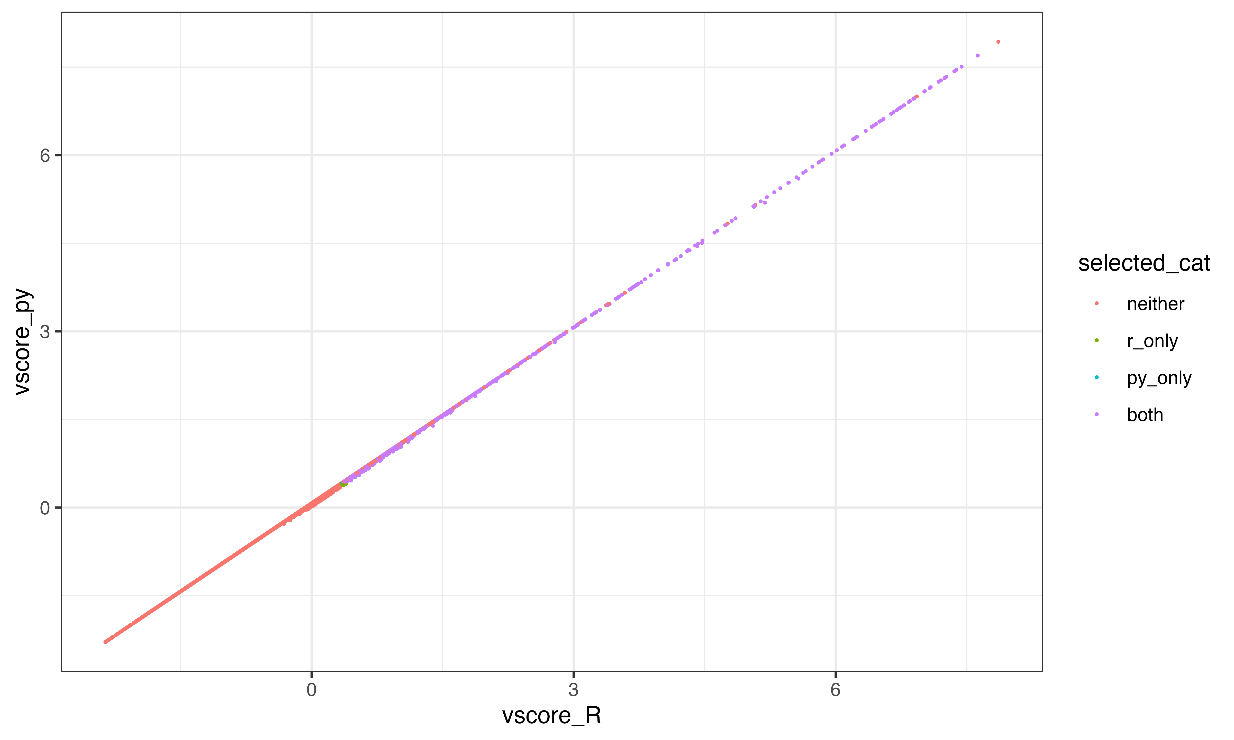
table(df$selected_cat)##
## neither r_only py_only both
## 22149 10 5 2472Highly variant features using R method
scr$pipeline_get_gene_filter(plot = TRUE)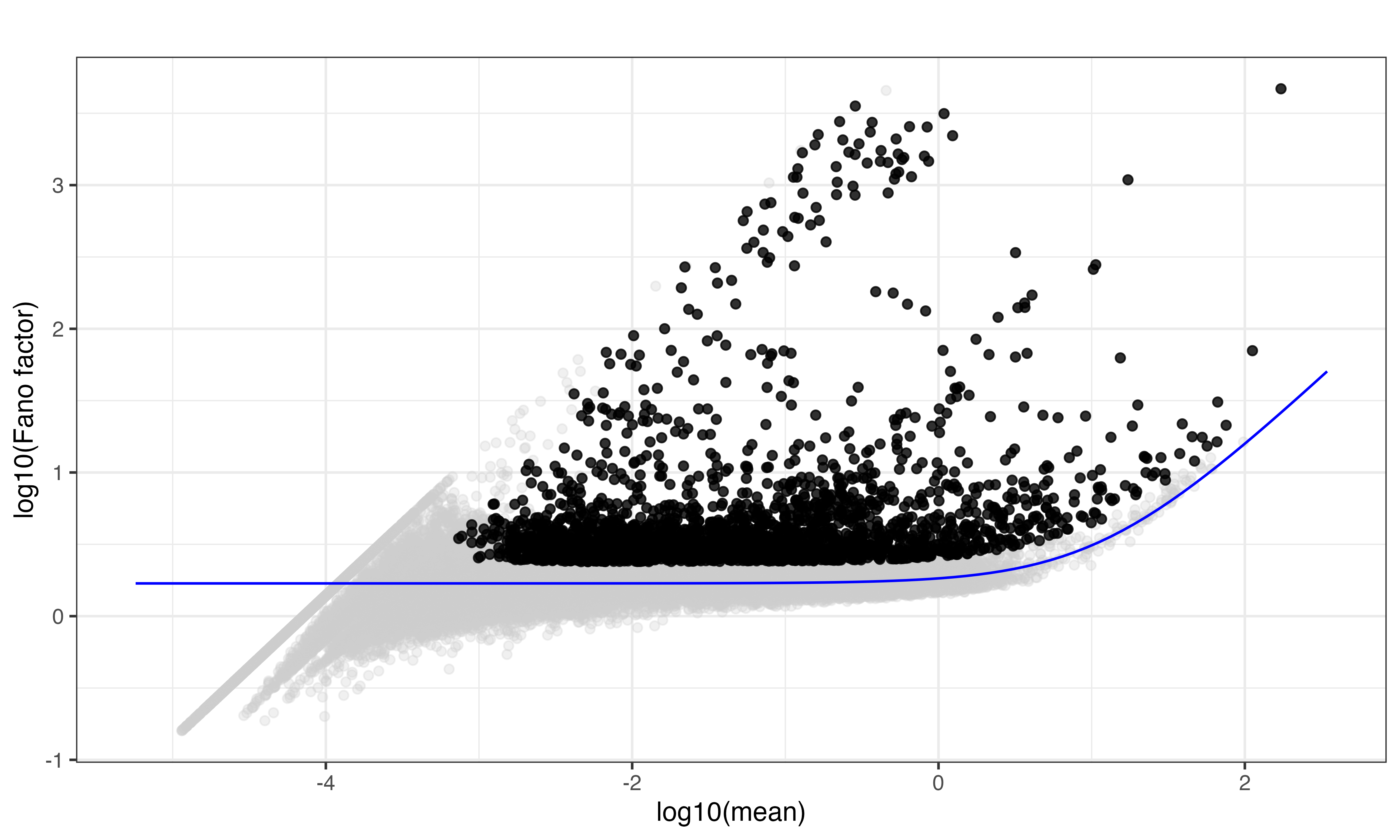
scr$pipeline_apply_gene_filter()Simulating doublets
sim_doublet_ratio = 2.0
synthetic_doublet_umi_subsampling = 1.0

scr$simulate_doublets(sim_doublet_ratio=sim_doublet_ratio, synthetic_doublet_umi_subsampling=synthetic_doublet_umi_subsampling)

scr$pipeline_normalize(postnorm_total=1e6)
scr.pipeline_get_gene_filter(scrub)
scr.pipeline_apply_gene_filter(scrub)
scrub.simulate_doublets(sim_doublet_ratio=scrub.sim_doublet_ratio, synthetic_doublet_umi_subsampling=synthetic_doublet_umi_subsampling)
scr.pipeline_normalize(scrub, postnorm_total=1e6)
r.py_Esimnorm = scrub._E_sim_norm
gene_filter = scrub._gene_filter
r.py_E_obs_norm = scrub._E_obs_norm
import copy
scrub_preZ = copy.deepcopy(scrub)Let’s umap
Here we will brind the pseudo doublets with the original count matrix and visualize using UMAP across the two implemnetations. They look similar.
library(magrittr)
rcounts<-t(rbind(scr$E_obs_norm, scr$E_sim_norm))
rownames(rcounts)<-rownames(seuP)[scr$gene_filter]
colnames(rcounts)<-1:dim(rcounts)[2]
seuR<-CreateSeuratObject(rcounts, meta.data = data.frame(celltype=c(as.character(seuP$celltype), rep("pseudodoublet", length(seuP$celltype)*2)), row.names = colnames(rcounts)))
seuR <-NormalizeData(seuR) %>% FindVariableFeatures(nfeatures = 1000) %>% ScaleData() %>% RunPCA(npcs = 50)
ElbowPlot(seuR, 50) 
seuR<- FindNeighbors(seuR, dims = 1:30) %>% FindClusters() %>% RunUMAP(dims = 1:30)## Modularity Optimizer version 1.3.0 by Ludo Waltman and Nees Jan van Eck
##
## Number of nodes: 41742
## Number of edges: 1409152
##
## Running Louvain algorithm...
## Maximum modularity in 10 random starts: 0.8846
## Number of communities: 27
## Elapsed time: 8 seconds
DimPlot(seuR, group.by = "celltype", cols = as.character(pals::polychrome(20))[c(1,3:16,2)], alpha = 0.1)+ggtitle("scrubletR")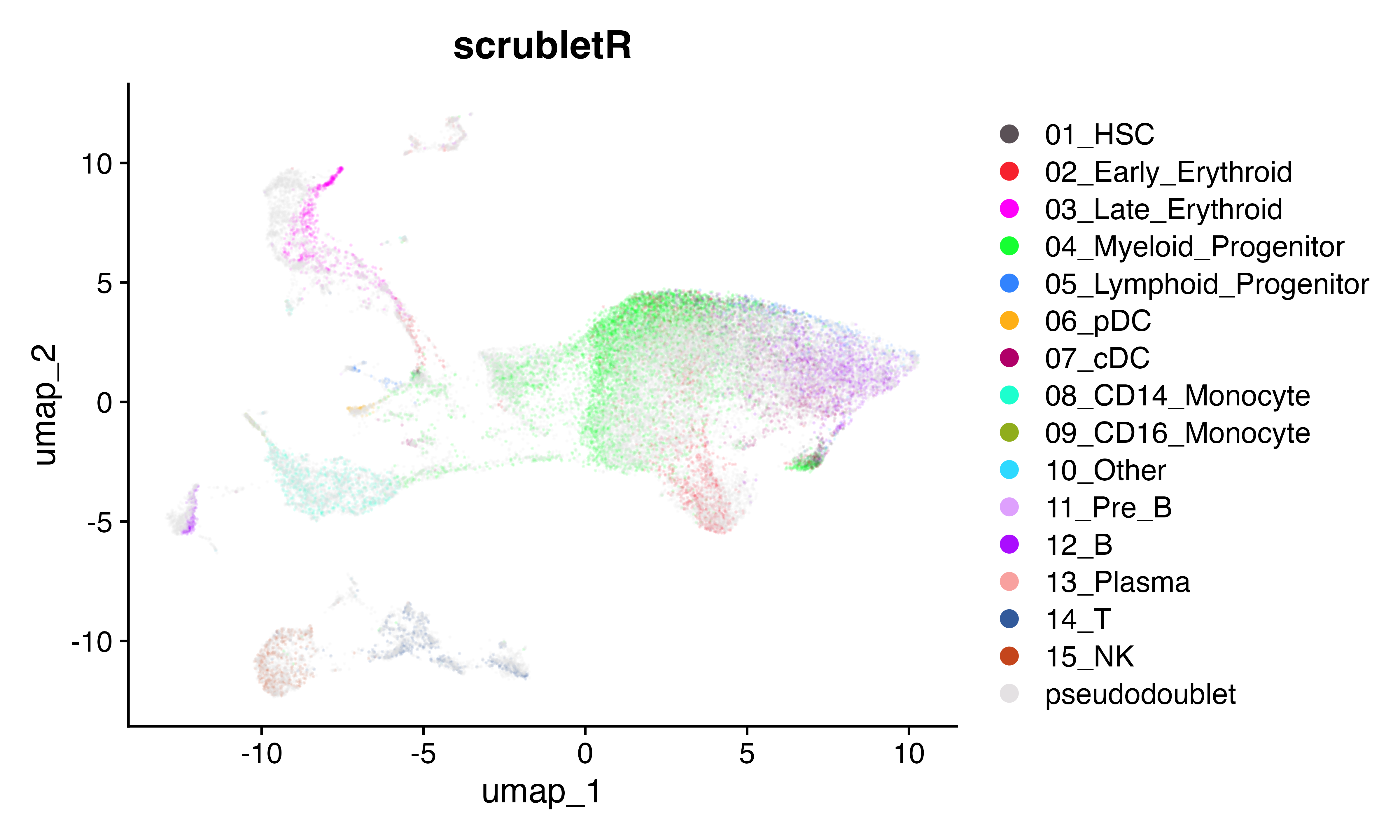
pycounts<-t(rbind(py_E_obs_norm, py_Esimnorm))
rownames(pycounts)<-rownames(seuP)[py$gene_filter]
colnames(pycounts)<-1:dim(pycounts)[2]
seuPy<-CreateSeuratObject(pycounts, meta.data = data.frame(celltype=c(as.character(seuP$celltype), rep("pseudodoublet", length(seuP$celltype)*2)), row.names = colnames(pycounts)))
seuPy <-NormalizeData(seuPy) %>% FindVariableFeatures(nfeatures = 1000) %>% ScaleData() %>% RunPCA(npcs = 50)
ElbowPlot(seuPy, 50) 
seuPy<- FindNeighbors(seuPy, dims = 1:40) %>% FindClusters() %>% RunUMAP(dims = 1:40)## Modularity Optimizer version 1.3.0 by Ludo Waltman and Nees Jan van Eck
##
## Number of nodes: 41742
## Number of edges: 1477580
##
## Running Louvain algorithm...
## Maximum modularity in 10 random starts: 0.8791
## Number of communities: 25
## Elapsed time: 8 seconds
DimPlot(seuPy, group.by = "celltype", cols = as.character(pals::polychrome(20))[c(1,3:16,2)], alpha = 0.1)+ggtitle("Scrublet (python)")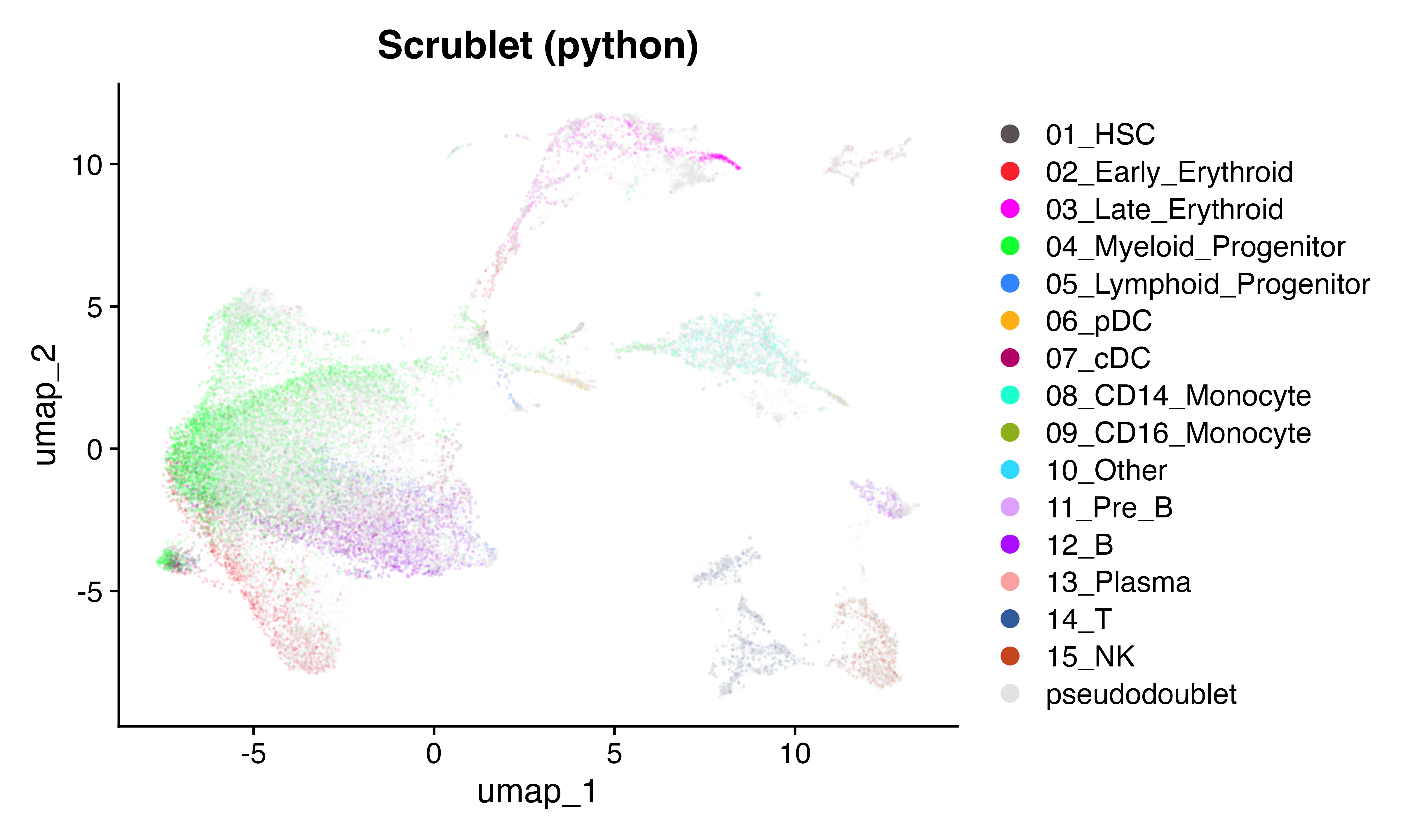
step by step
Step 1 calculate gene mean and stdev
These look pretty similar
gene_mean = as.numeric(colMeans(scr$E_obs_norm)) #######changed to column - IS CORRECT
gene_stdev = as.numeric(sqrt(scrubletR:::sparse_var(scr$E_obs_norm, axis = 2)))
# print_py(gene_mean)
# print_py(gene_stdev)
# print_py(py$gene_means[1,])
# print_py(py$gene_stdevs)

ggplot(data.frame(mean=log(c(gene_mean, py$gene_means[1,])), stdev=log(c(gene_stdev, py$gene_stdevs)), impl=c(rep("R", length(gene_mean)), rep("Py", length(py$gene_means)))), aes(x=mean, fill=impl))+geom_density()+theme_bw()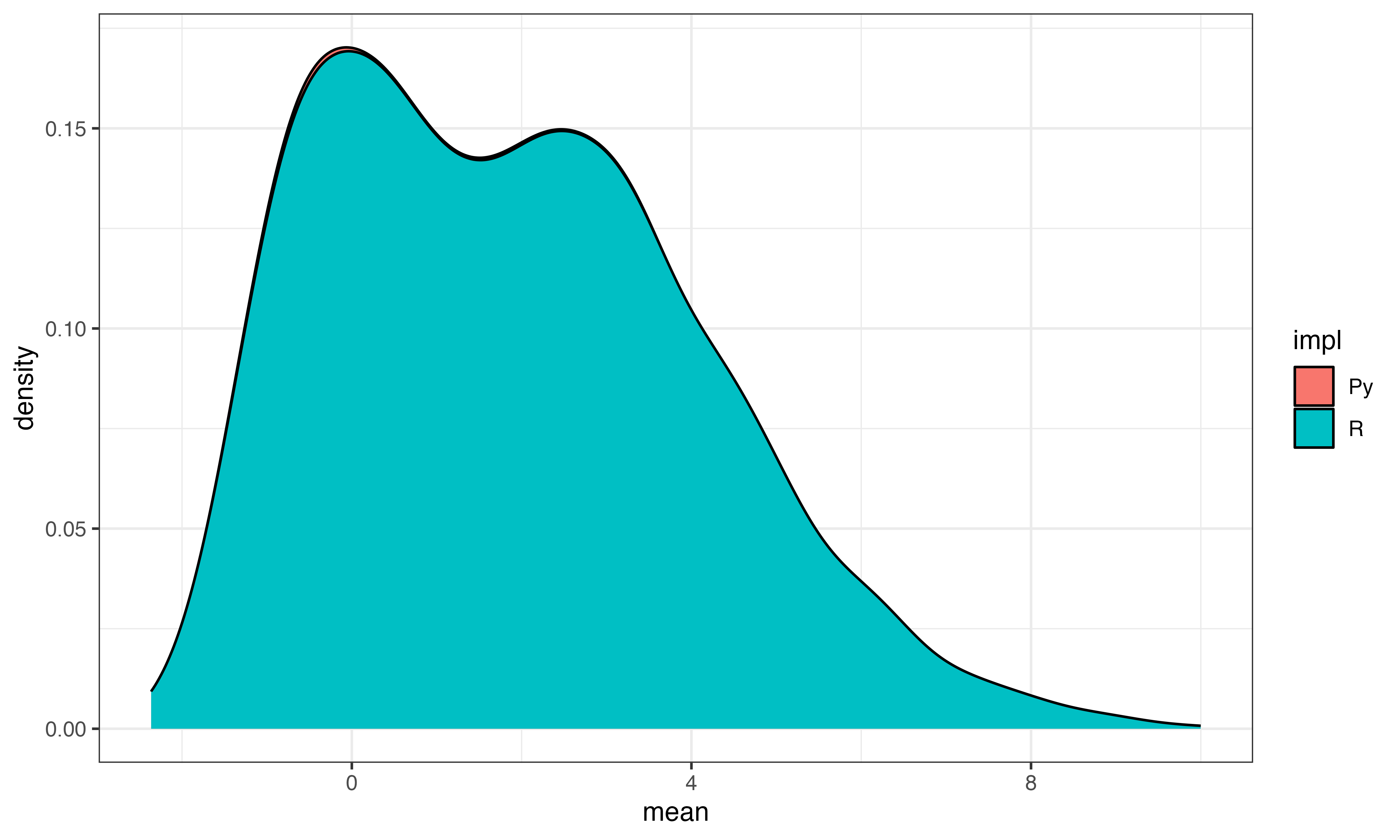
ggplot(data.frame(mean=log(c(gene_mean, py$gene_means[1,])), stdev=log(c(gene_stdev, py$gene_stdevs)), impl=c(rep("R", length(gene_mean)), rep("Py", length(py$gene_means)))), aes(x=stdev, fill=impl))+geom_density()+theme_bw()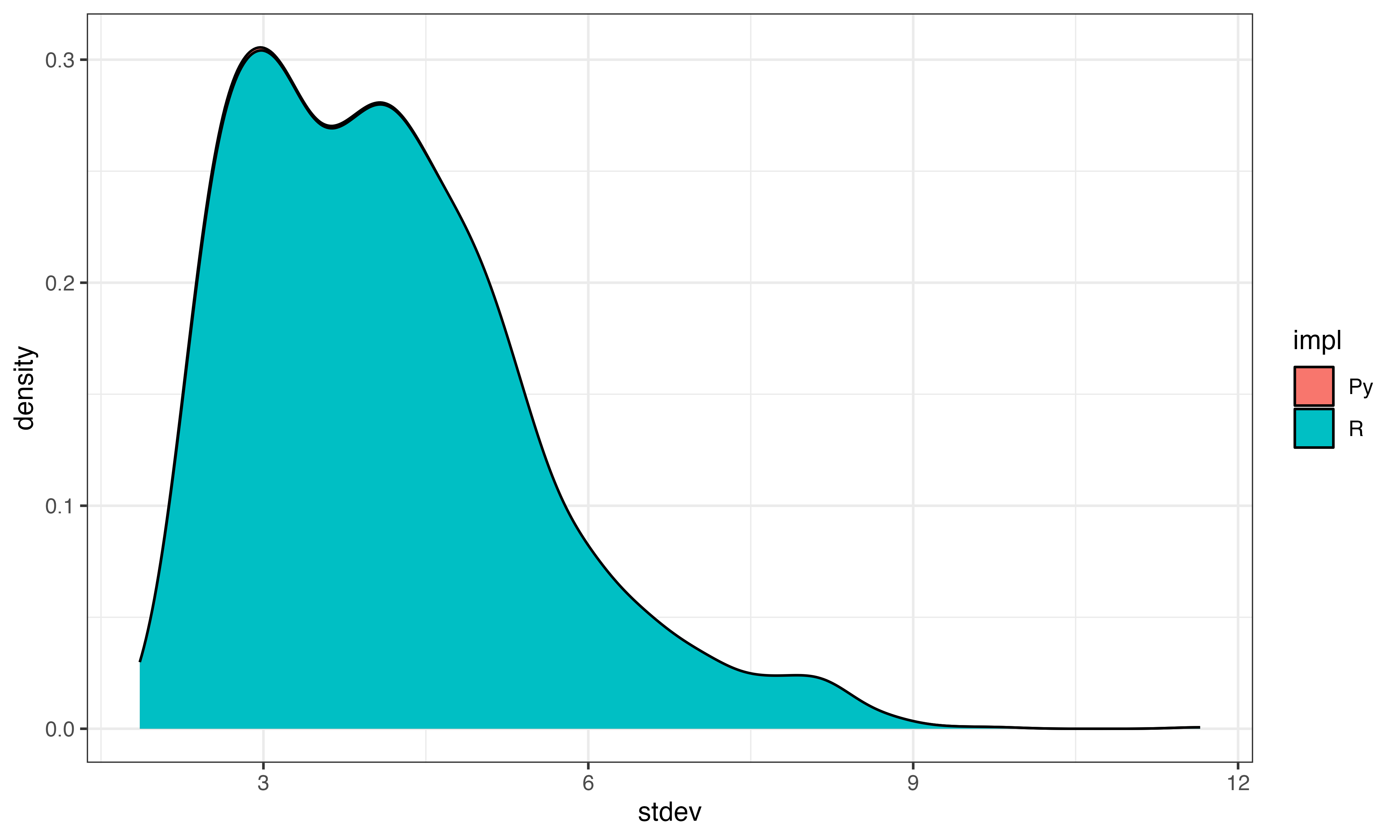
#(same as py)Step 2 subtract gene means
preZ_Eobs_norm = scrub_preZ._E_obs_norm
step2 = preZ_Eobs_norm - preZ_Eobs_norm.mean(0) # this step is easy in python
Here’s what you get in R with similarly structured code
step2 = scr$E_obs_norm - colMeans(scr$E_obs_norm) # this doesn't work as intended in R
colnames(step2)<-NULL

step2[1:5,1:5]
## 5 x 5 Matrix of class "dgeMatrix"
## [,1] [,2] [,3] [,4] [,5]
## [1,] -1.0294501 -1.281551 -6.4029111 -3.358221 -2.5414889
## [2,] -0.1149148 -2.725418 -47.6427631 98.450927 -202.0442150
## [3,] -0.5069102 -26.156322 -7.0442071 -4.829656 -158.6784346
## [4,] -47.4869206 -4.985819 -0.4297543 -57.322949 -0.5091509
## [5,] -2.7516240 -483.210268 -76.2160384 -7.571018 -3.4020053
py$step2[1:5,1:5]## [,1] [,2] [,3] [,4] [,5]
## [1,] -1.02945 -0.1149148 -0.5069102 -47.48692 -2.751624
## [2,] -1.02945 -0.1149148 -0.5069102 52.62320 -2.751624
## [3,] -1.02945 -0.1149148 -0.5069102 -47.48692 -2.751624
## [4,] -1.02945 -0.1149148 -0.5069102 -47.48692 -2.751624
## [5,] -1.02945 -0.1149148 -0.5069102 -47.48692 -2.751624Turns out R has some peculiarities and for subtracting a vector element-wise from the column values of matrix we must first create a matrix duplicating the desired subtracted values down all the rows. Simply subtracting the vector (in this case of gene means from each column (gene) of the matrix cannot be done using simply matrix - vector) In python, the subtraction using numpy is much easier…
sm<-matrix(rep(colMeans(scr$E_obs_norm), each = dim(scr$E_obs_norm)[1]), nrow=dim(scr$E_obs_norm)[1])
step2 = scr$E_obs_norm - sm
colnames(step2)<-NULL
step2[1:5,1:5]## 5 x 5 Matrix of class "dgeMatrix"
##          [,1]       [,2]       [,3]      [,4]      [,5]
## [1,] -1.02945 -0.1149148 -0.5069102 -47.48692 -2.751624
## [2,] -1.02945 -0.1149148 -0.5069102  52.62320 -2.751624
## [3,] -1.02945 -0.1149148 -0.5069102 -47.48692 -2.751624
## [4,] -1.02945 -0.1149148 -0.5069102 -47.48692 -2.751624
## [5,] -1.02945 -0.1149148 -0.5069102 -47.48692 -2.751624
py$step2[1:5,1:5]## [,1] [,2] [,3] [,4] [,5]
## [1,] -1.02945 -0.1149148 -0.5069102 -47.48692 -2.751624
## [2,] -1.02945 -0.1149148 -0.5069102 52.62320 -2.751624
## [3,] -1.02945 -0.1149148 -0.5069102 -47.48692 -2.751624
## [4,] -1.02945 -0.1149148 -0.5069102 -47.48692 -2.751624
## [5,] -1.02945 -0.1149148 -0.5069102 -47.48692 -2.751624Step 3 complete zscoring
Looks good
step3<-t(scrubletR:::sparse_multiply(t(step2), 1 / gene_stdev))

ggplot(data.frame(x=rowMeans(step3), y=rowMeans(py$step3)), aes(x=x, y=y))+geom_point()+theme_bw()+xlab("R rowMeans of Step3")+ylab("Python rowMeans of Step3")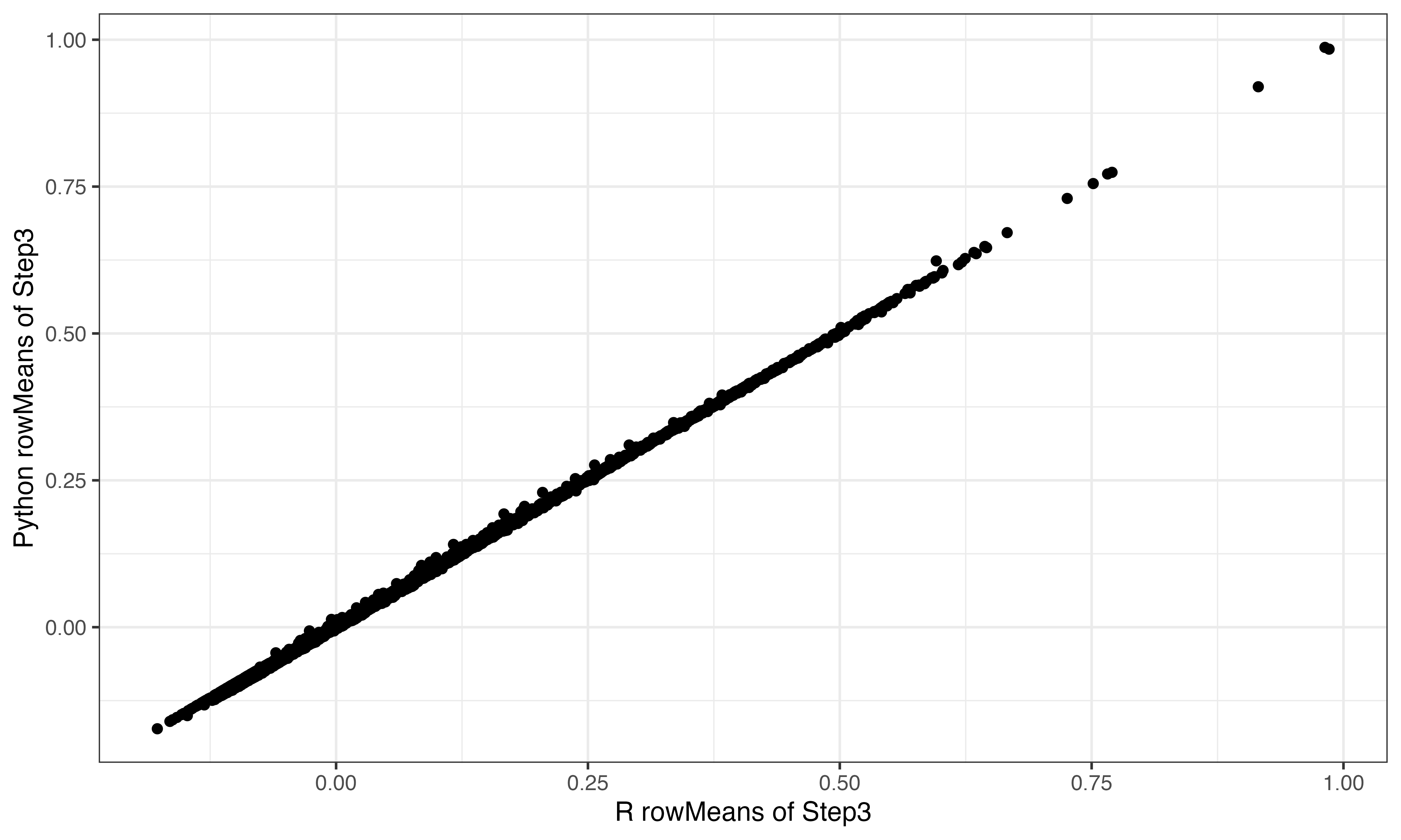
scr$pipeline_zscore()Step 4 PCA
import scipy
from sklearn.decomposition import PCA
X_obs = scrub._E_obs_norm
X_sim = scrub._E_sim_norm

pca = PCA(n_components=n_prin_comps, random_state=random_state, svd_solver=svd_solver).fit(X_obs)

pto = pca.transform(X_obs)
pts = pca.transform(X_sim)
X_obs <- as.matrix(scr$E_obs_norm)
X_sim <- as.matrix(scr$E_sim_norm)
pca <- irlba::prcomp_irlba(X_obs, n = n_prin_comps, center = TRUE, scale. = FALSE)


ix<-sample(1:nrow(X_obs), 2000)


ggplot(data.frame(py = abs(py$pto[ix,1]), R = abs(predict(pca, X_obs)[ix,1])), aes(x=R, y=py))+geom_point()+theme_bw()+ggtitle("Correlation of R and Python PC1 values (Obs)")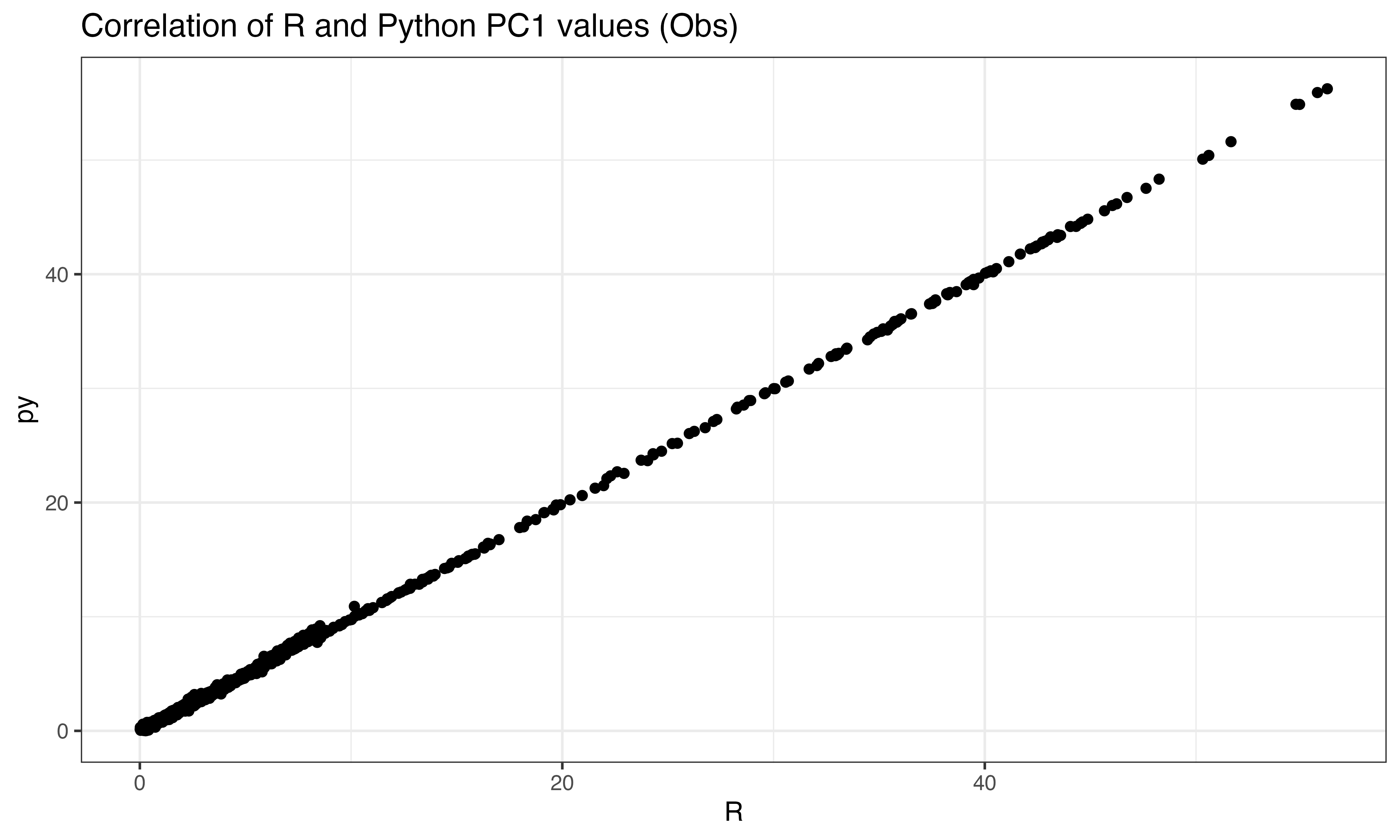
ggplot(data.frame(py = abs(py$pto[ix,2]), R = abs(predict(pca, X_obs)[ix,2])), aes(x=R, y=py))+geom_point()+theme_bw()+ggtitle("Correlation of R and Python PC2 values (Obs)")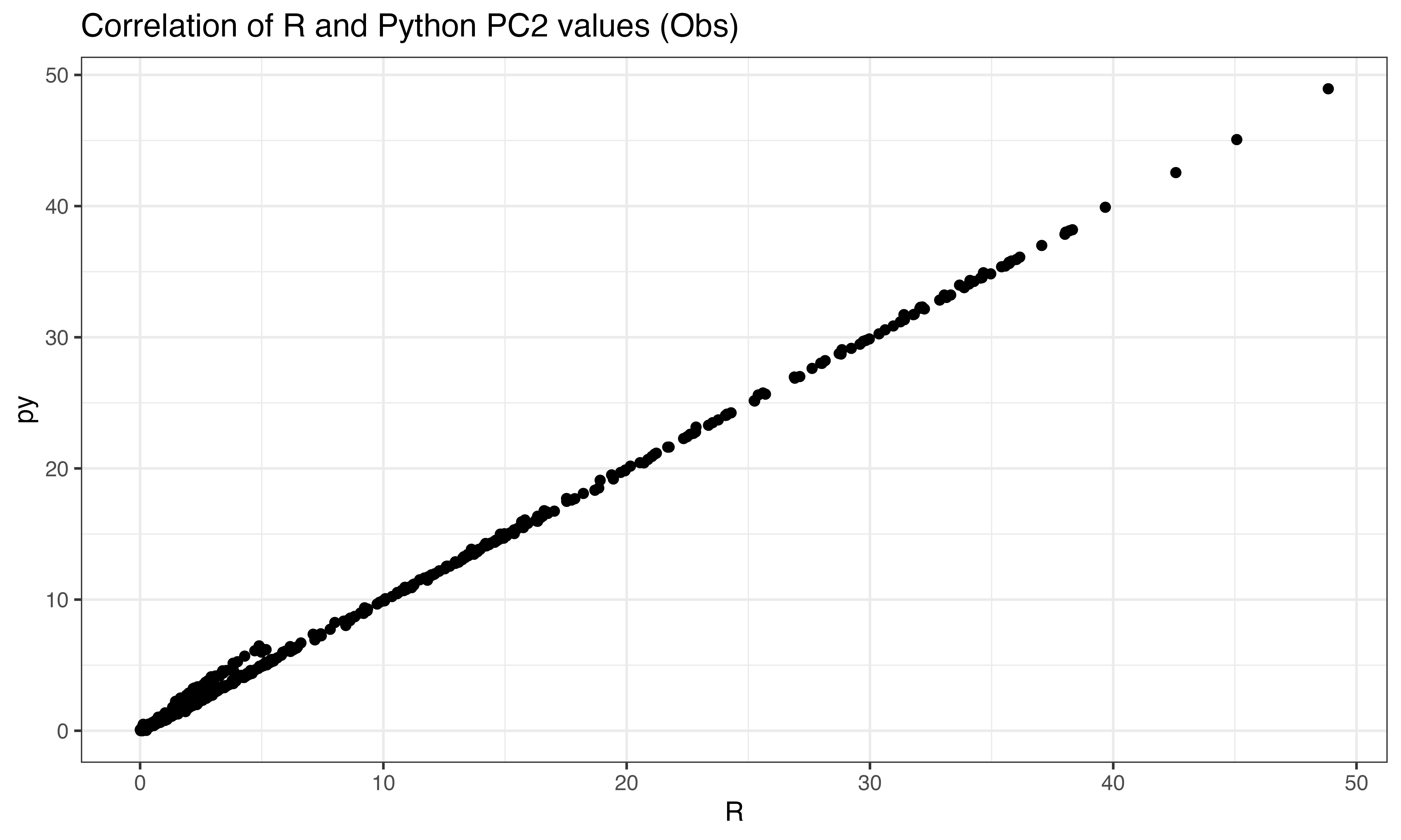
ggplot(data.frame(py = abs(py$pto[ix,3]), R = abs(predict(pca, X_obs)[ix,3])), aes(x=R, y=py))+geom_point()+theme_bw()+ggtitle("Correlation of R and Python PC3 values (Obs)")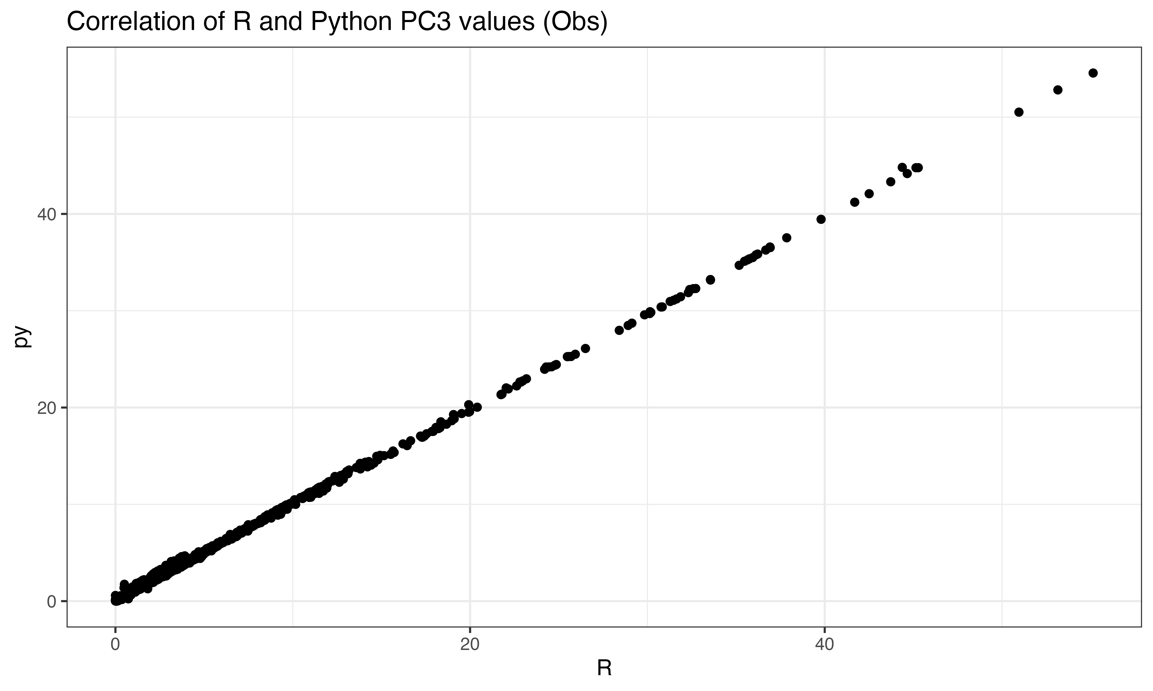
#these should not be correlated (Simulated data)
ggplot(data.frame(py = abs(py$pts[ix,1]), R = abs(predict(pca, X_sim)[ix,1])), aes(x=R, y=py))+geom_point()+theme_bw()+ggtitle("Correlation of R and Python PC1 values (Sim)")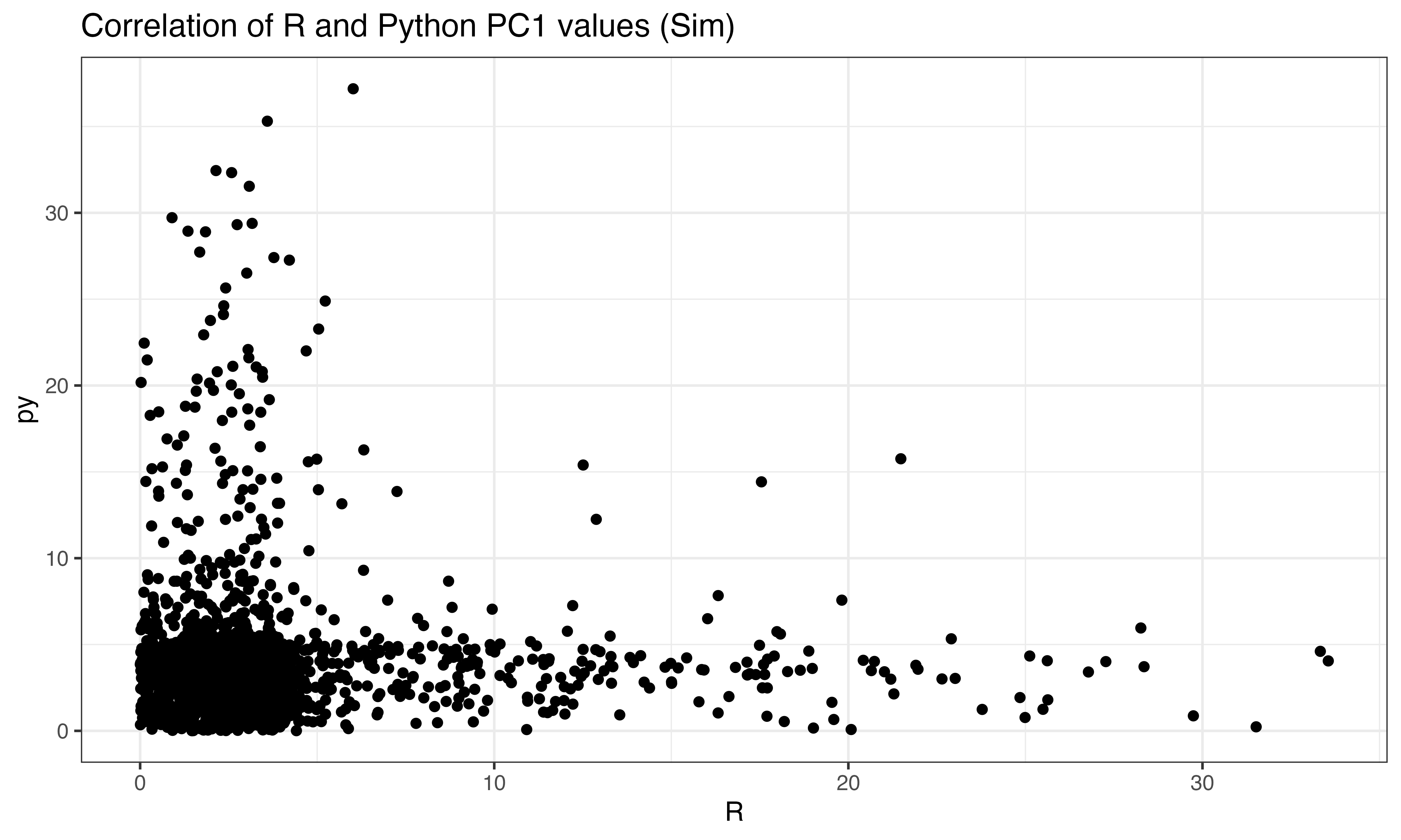
ggplot(data.frame(py = abs(py$pts[ix,2]), R = abs(predict(pca, X_sim)[ix,2])), aes(x=R, y=py))+geom_point()+theme_bw()+ggtitle("Correlation of R and Python PC2 values (Sim)")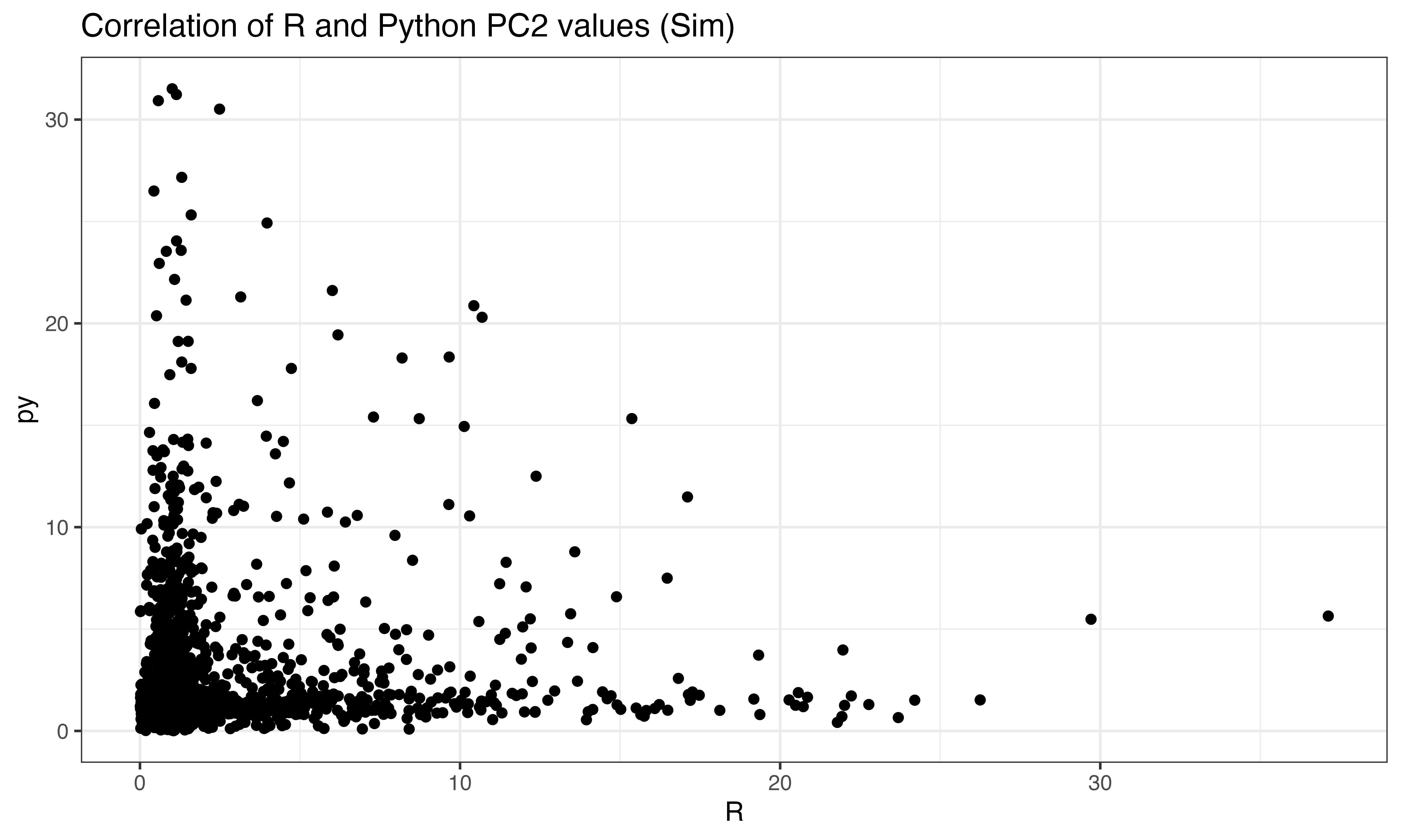
ggplot(data.frame(py = abs(py$pts[ix,3]), R = abs(predict(pca, X_sim)[ix,3])), aes(x=R, y=py))+geom_point()+theme_bw()+ggtitle("Correlation of R and Python PC3 values (Sim)")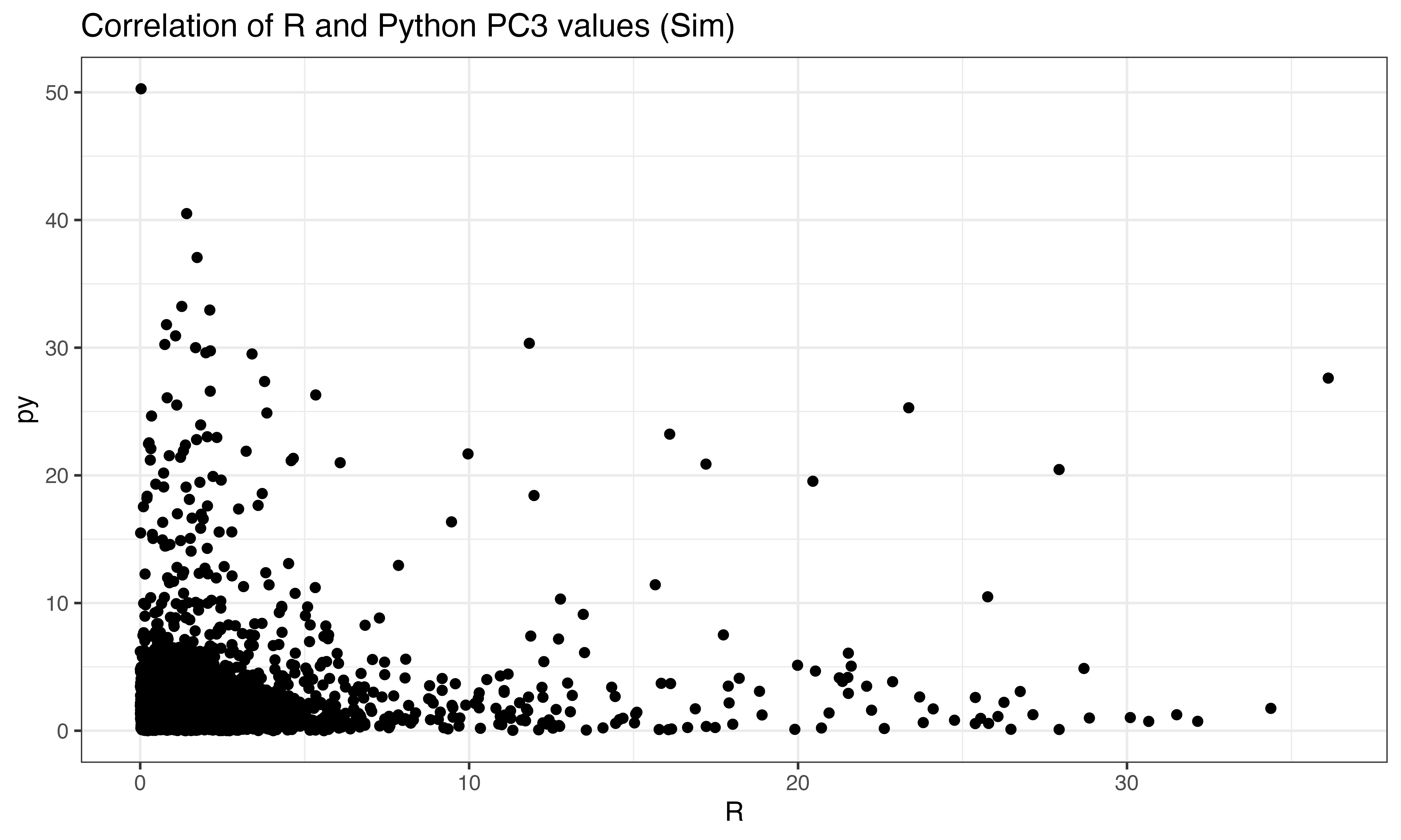
Step 4 calculate doublet scores
scr$pipeline_pca()
scr$calculate_doublet_scores()
scr.pipeline_pca(scrub)
scrub.calculate_doublet_scores(
use_approx_neighbors=use_approx_neighbors,
distance_metric=distance_metric,
get_doublet_neighbor_parents=get_doublet_neighbor_parents
)## array([0.05319149, 0.0928 , 0.06432749, ..., 0.07152682, 0.11666667,
## 0.21625544])Interesting that the tumor shows less correlation across the two implementations than other celltypes
ggplot(data.frame(py = log(py$final_doublet), R = log(scr$doublet_scores_obs_), celltype = seuP$celltype), aes(x=R, y=py, color = celltype))+geom_point(size = 0.3)+theme_bw()+ggtitle("Correlation of R and Python doublet scores (log transformed)")+scale_color_manual(values = as.character(pals::polychrome()))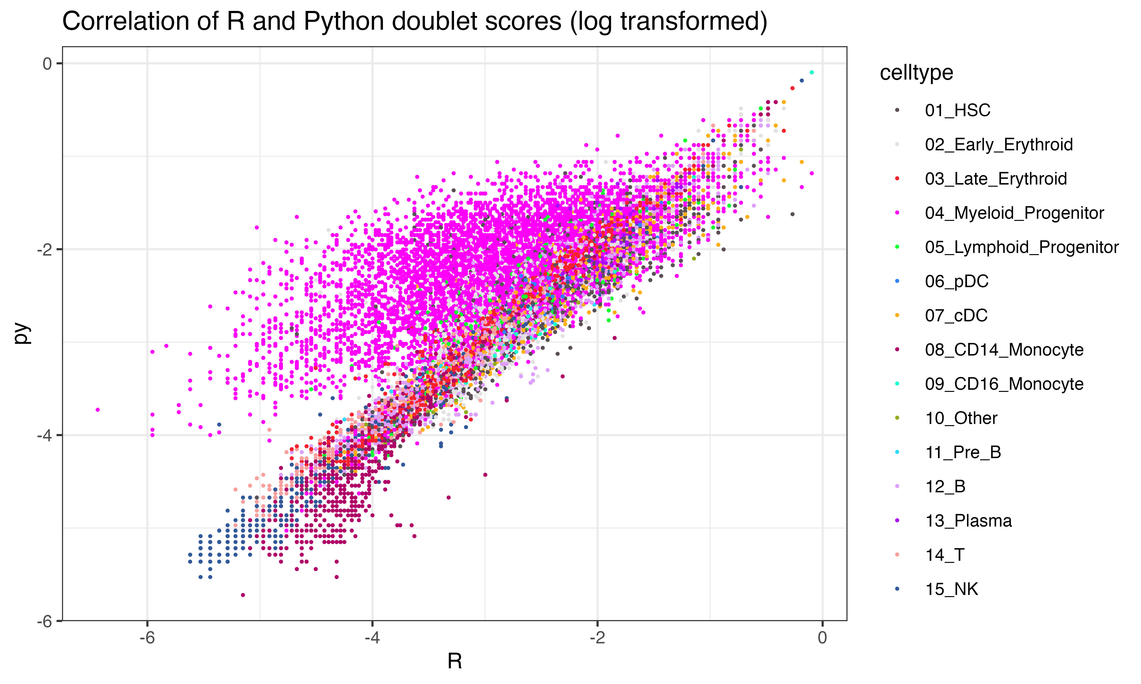
ggplot(data.frame(py = log(py$final_doublet), R = log(scr$doublet_scores_obs_), genotype = seuP$geno), aes(x=R, y=py, color = genotype))+geom_point(size = 0.3, alpha = 0.3)+theme_bw()+ggtitle("Correlation of R and Python doublet scores (log transformed)")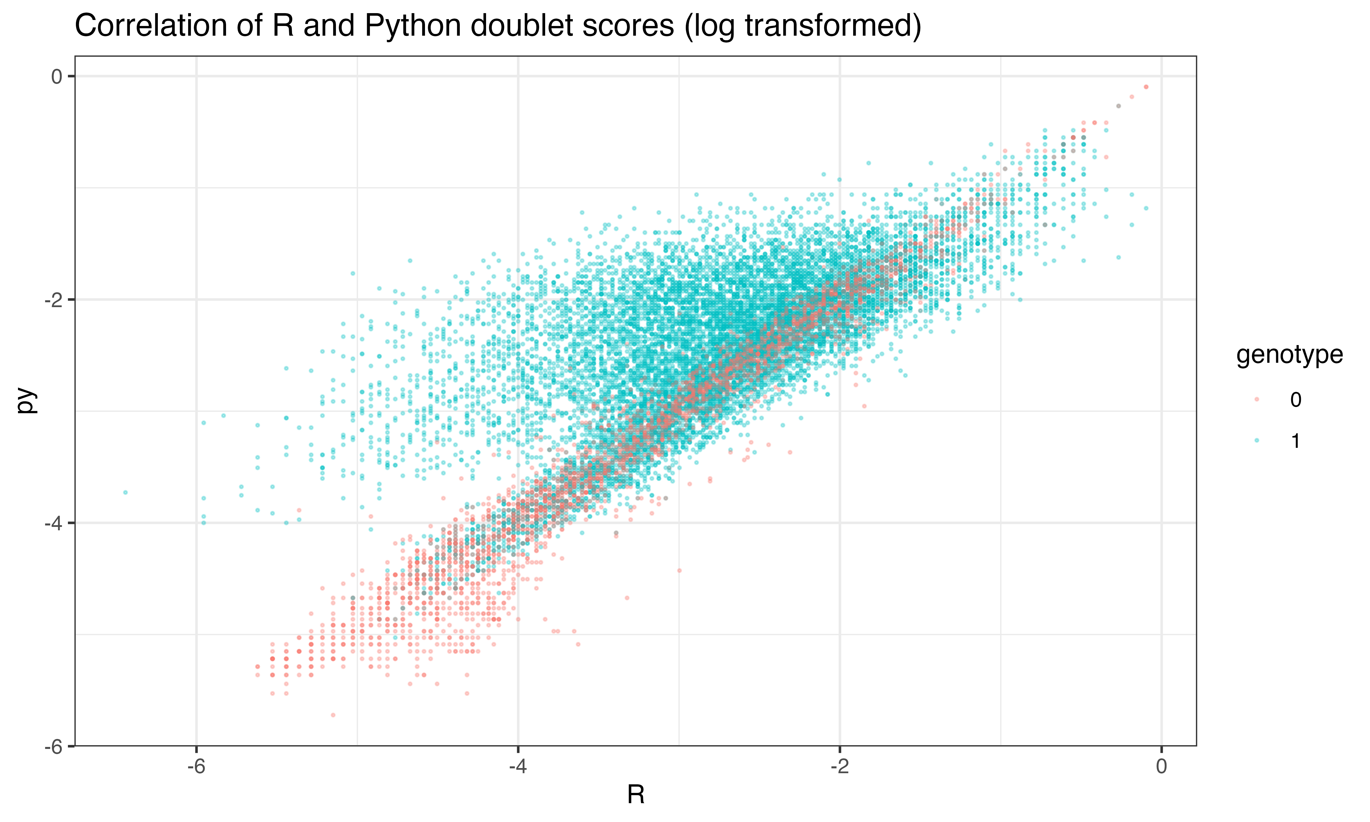
Step 5 Classify doublets
Not bad… 98.67% accurate… This may be related to the differences in features but also the python implementation calls a lower number of doubles overall…
## Automatically set threshold at doublet score = 0.68
## Detected doublet rate = 0.0%
## Estimated detectable doublet fraction = 14.2%
## Overall doublet rate:
##  Expected   = 10.0%
##  Estimated  = 0.3%
## array([False, False, False, ..., False, False, False])
scr$call_doublets()
confusion_matrix(factor(scr$predicted_doublets), factor(py$pred_doublets))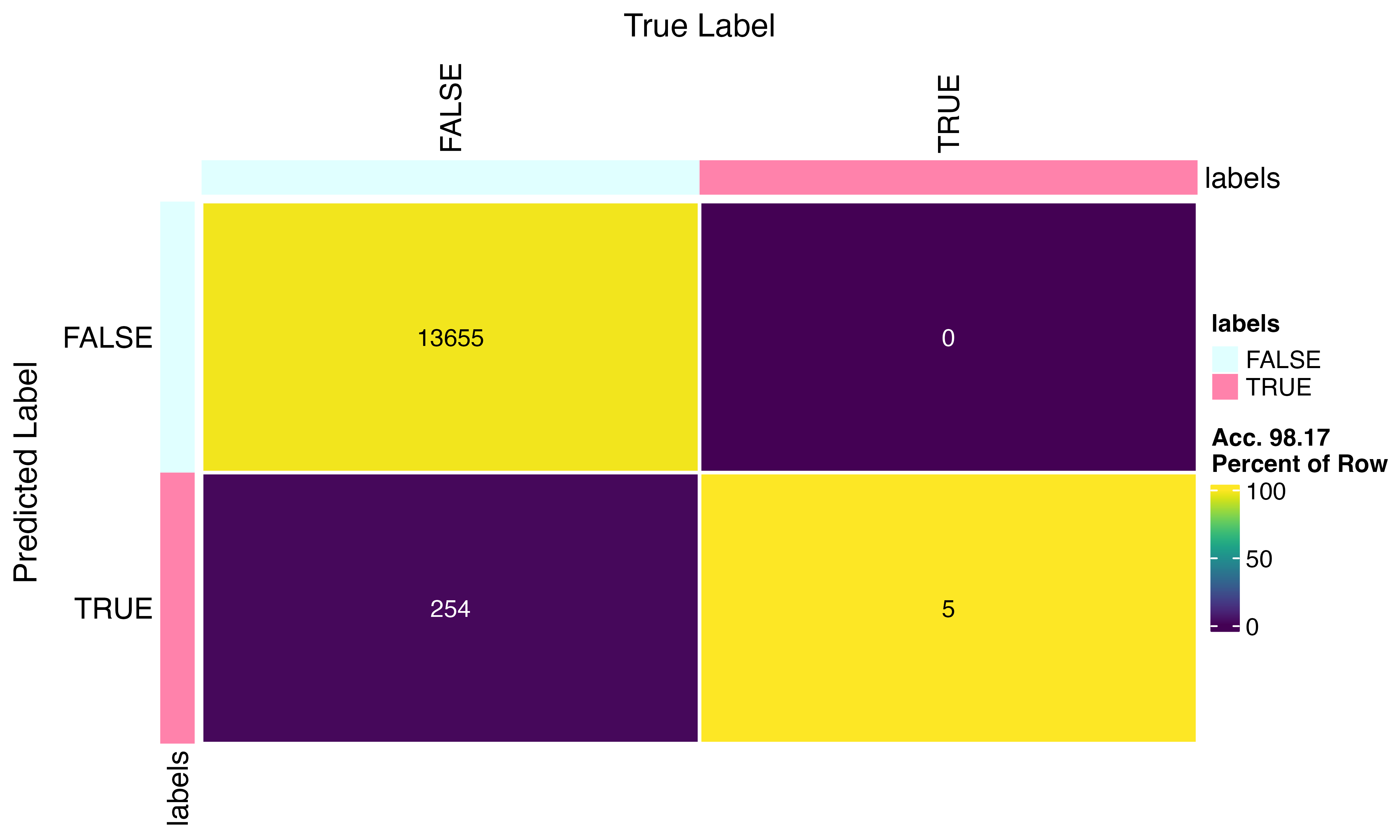
Level the playing field
Let’s rerun R scrublet using the python gene filter…
gene_filter = scrub._gene_filter
E_sim = scrub._E_sim
doublet_parents = scrub.doublet_parents_
tots_sim = scrub._total_counts_sim
#instantiate object
scr<-ScrubletR$new(counts_matrix = counts_matrix)
scr$pipeline_normalize()
new_gene_filter<-py$gene_filter+1
names(new_gene_filter)<-colnames(counts_matrix)[new_gene_filter]

scr$E_obs <- scr$E_obs[, as.numeric(new_gene_filter)]
scr$E_obs_norm <- scr$E_obs_norm[, as.numeric(new_gene_filter)]

scr$simulate_doublets(sim_doublet_ratio=1, synthetic_doublet_umi_subsampling=1)
scr$pipeline_normalize(postnorm_total=1e6)
scr$pipeline_zscore()
scr$pipeline_pca()
scr$calculate_doublet_scores()
scr$call_doublets()
ggplot(data.frame(py = log(py$final_doublet), R = log(scr$doublet_scores_obs_), celltype = seuP$celltype), aes(x=R, y=py, color = celltype))+geom_point(size = 0.3)+theme_bw()+ggtitle("Correlation of R and Python doublet scores (log transformed) using same features set")+scale_color_manual(values = as.character(pals::polychrome()))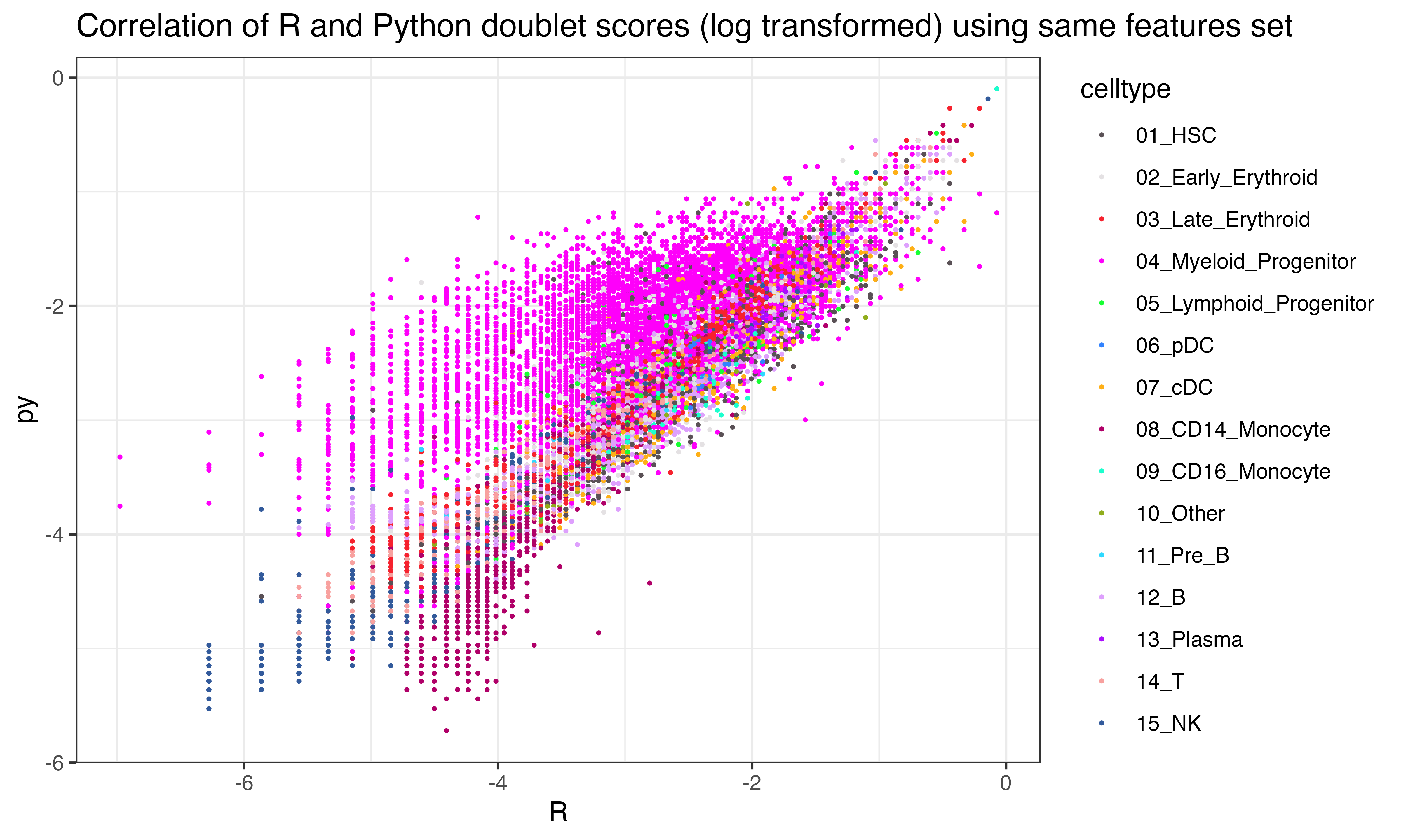
confusion_matrix(factor(scr$predicted_doublets), factor(py$pred_doublets))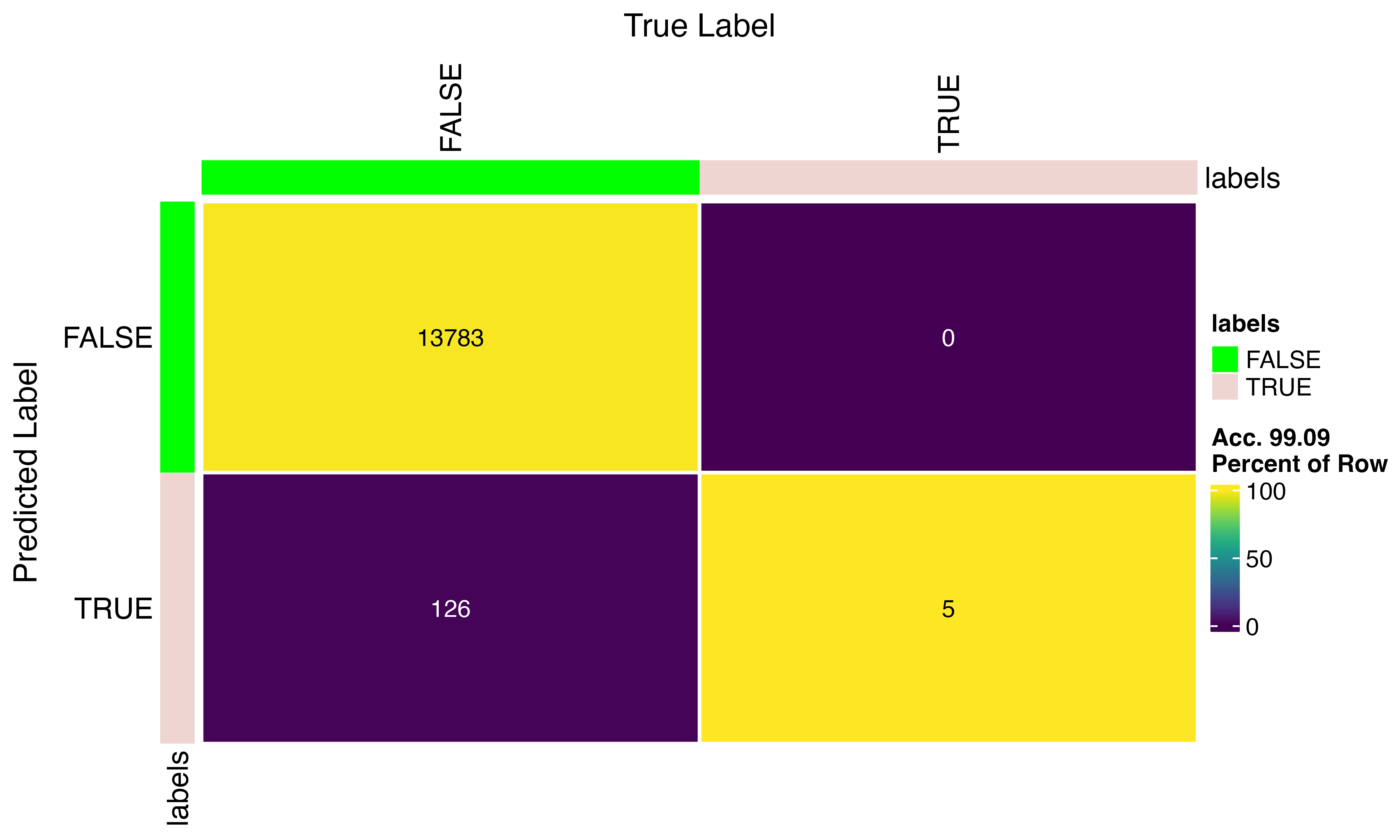
#instantiate object
scr<-ScrubletR$new(counts_matrix = counts_matrix)
scr$pipeline_normalize()
new_gene_filter<-py$gene_filter+1
names(new_gene_filter)<-colnames(counts_matrix)[new_gene_filter]

scr$E_obs <- scr$E_obs[, as.numeric(new_gene_filter)]
scr$E_obs_norm <- scr$E_obs_norm[, as.numeric(new_gene_filter)]

dim(scr$E_obs)
## [1] 13914 2477
scr$total_counts_sim = py$tots_sim
scr$E_sim <- py$E_sim
scr$pipeline_normalize(postnorm_total=1e6)
scr$pipeline_zscore()
scr$pipeline_pca()
scr$calculate_doublet_scores()
scr$call_doublets()
ggplot(data.frame(py = log(py$final_doublet), R = log(scr$doublet_scores_obs_), celltype = seuP$celltype), aes(x=R, y=py, color = celltype))+geom_point(size = 0.3)+theme_bw()+ggtitle("Correlation of R and Python doublet scores (log transformed) using same features and same simulated doublets")+scale_color_manual(values = as.character(pals::polychrome()))
confusion_matrix(factor(scr$predicted_doublets), factor(py$pred_doublets))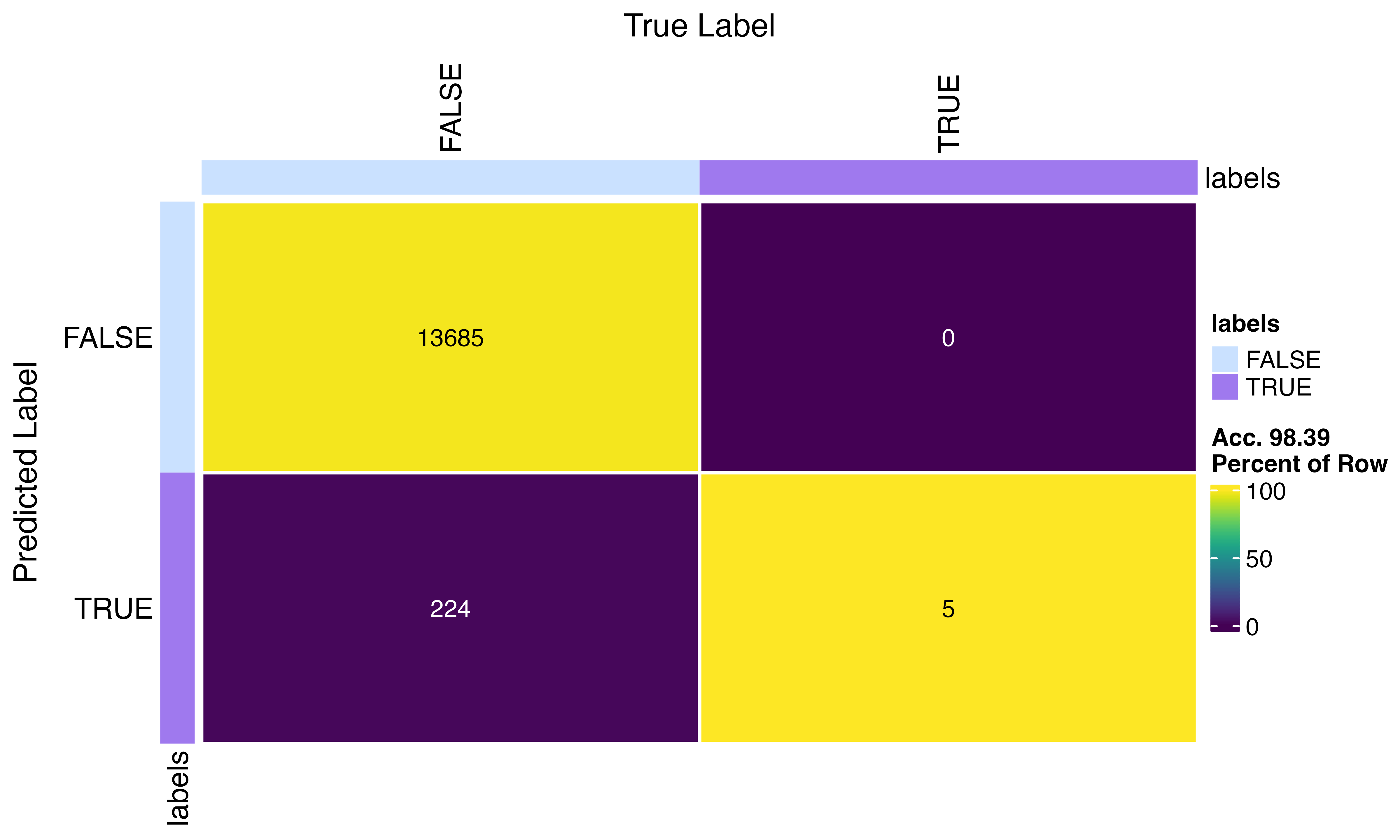
Appendix
## R version 4.3.1 (2023-06-16)
## Platform: x86_64-apple-darwin20 (64-bit)
## Running under: macOS Ventura 13.6.3
##
## Matrix products: default
## BLAS:   /Library/Frameworks/R.framework/Versions/4.3-x86_64/Resources/lib/libRblas.0.dylib
## LAPACK: /Library/Frameworks/R.framework/Versions/4.3-x86_64/Resources/lib/libRlapack.dylib;  LAPACK version 3.11.0
##
## locale:
## [1] en_US.UTF-8/en_US.UTF-8/en_US.UTF-8/C/en_US.UTF-8/en_US.UTF-8
##
## time zone: America/Los_Angeles
## tzcode source: internal
##
## attached base packages:
## [1] stats     graphics  grDevices utils     datasets  methods   base
##
## other attached packages:
##  [1] magrittr_2.0.3     ggplot2_3.4.4      Matrix_1.6-5       scCustomize_2.0.1
##  [5] Seurat_5.0.1.9004  SeuratObject_5.0.1 sp_2.1-3           viewmastR_0.2.1
##  [9] scrubletR_0.2.0    reticulate_1.35.0
##
## loaded via a namespace (and not attached):
##   [1] fs_1.6.3                    matrixStats_1.2.0
##   [3] spatstat.sparse_3.0-3       bitops_1.0-7
##   [5] RcppMsgPack_0.2.3           lubridate_1.9.3
##   [7] httr_1.4.7                  RColorBrewer_1.1-3
##   [9] doParallel_1.0.17           tools_4.3.1
##  [11] sctransform_0.4.1           backports_1.4.1
##  [13] utf8_1.2.4                  R6_2.5.1
##  [15] lazyeval_0.2.2              uwot_0.1.16
##  [17] GetoptLong_1.0.5            withr_3.0.0
##  [19] gridExtra_2.3               progressr_0.14.0
##  [21] cli_3.6.2                   Biobase_2.60.0
##  [23] textshaping_0.3.7           Cairo_1.6-2
##  [25] spatstat.explore_3.2-6      fastDummies_1.7.3
##  [27] labeling_0.4.3              prismatic_1.1.1
##  [29] sass_0.4.8                  spatstat.data_3.0-4
##  [31] proxy_0.4-27                ggridges_0.5.6
##  [33] pbapply_1.7-2               pkgdown_2.0.7
##  [35] systemfonts_1.0.5           foreign_0.8-86
##  [37] dichromat_2.0-0.1           parallelly_1.36.0
##  [39] maps_3.4.2                  pals_1.8
##  [41] rstudioapi_0.15.0           generics_0.1.3
##  [43] shape_1.4.6                 ica_1.0-3
##  [45] spatstat.random_3.2-2       dplyr_1.1.4
##  [47] ggbeeswarm_0.7.2            fansi_1.0.6
##  [49] S4Vectors_0.38.2            abind_1.4-5
##  [51] lifecycle_1.0.4             yaml_2.3.8
##  [53] snakecase_0.11.1            SummarizedExperiment_1.30.2
##  [55] recipes_1.0.9               Rtsne_0.17
##  [57] paletteer_1.6.0             grid_4.3.1
##  [59] promises_1.2.1              crayon_1.5.2
##  [61] miniUI_0.1.1.1              lattice_0.22-5
##  [63] cowplot_1.1.3               mapproj_1.2.11
##  [65] pillar_1.9.0                knitr_1.45
##  [67] ComplexHeatmap_2.16.0       GenomicRanges_1.52.1
##  [69] rjson_0.2.21                boot_1.3-28.1
##  [71] future.apply_1.11.1         codetools_0.2-19
##  [73] leiden_0.4.3.1              glue_1.7.0
##  [75] data.table_1.15.0           vctrs_0.6.5
##  [77] png_0.1-8                   spam_2.10-0
##  [79] gtable_0.3.4                rematch2_2.1.2
##  [81] assertthat_0.2.1            cachem_1.0.8
##  [83] gower_1.0.1                 xfun_0.41
##  [85] S4Arrays_1.2.0              mime_0.12
##  [87] prodlim_2023.08.28          survival_3.5-7
##  [89] timeDate_4032.109           SingleCellExperiment_1.22.0
##  [91] iterators_1.0.14            pbmcapply_1.5.1
##  [93] hardhat_1.3.0               lava_1.7.3
##  [95] ellipsis_0.3.2              fitdistrplus_1.1-11
##  [97] ROCR_1.0-11                 ipred_0.9-14
##  [99] nlme_3.1-164                RcppAnnoy_0.0.22
## [101] GenomeInfoDb_1.36.4         bslib_0.6.1
## [103] irlba_2.3.5.1               vipor_0.4.7
## [105] KernSmooth_2.23-22          rpart_4.1.23
## [107] colorspace_2.1-0            BiocGenerics_0.46.0
## [109] Hmisc_5.1-1                 nnet_7.3-19
## [111] ggrastr_1.0.2               tidyselect_1.2.0
## [113] compiler_4.3.1              htmlTable_2.4.2
## [115] desc_1.4.3                  DelayedArray_0.26.7
## [117] plotly_4.10.4               checkmate_2.3.1
## [119] scales_1.3.0                lmtest_0.9-40
## [121] stringr_1.5.1               digest_0.6.34
## [123] goftest_1.2-3               spatstat.utils_3.0-4
## [125] minqa_1.2.6                 rmarkdown_2.25
## [127] XVector_0.40.0              htmltools_0.5.7
## [129] pkgconfig_2.0.3             base64enc_0.1-3
## [131] lme4_1.1-35.1               sparseMatrixStats_1.12.2
## [133] MatrixGenerics_1.12.3       highr_0.10
## [135] fastmap_1.1.1               rlang_1.1.3
## [137] GlobalOptions_0.1.2         htmlwidgets_1.6.4
## [139] shiny_1.8.0                 DelayedMatrixStats_1.22.6
## [141] farver_2.1.1                jquerylib_0.1.4
## [143] zoo_1.8-12                  jsonlite_1.8.8
## [145] ModelMetrics_1.2.2.2        RCurl_1.98-1.14
## [147] Formula_1.2-5               GenomeInfoDbData_1.2.10
## [149] dotCall64_1.1-1             patchwork_1.2.0
## [151] munsell_0.5.0               Rcpp_1.0.12
## [153] stringi_1.8.3               pROC_1.18.5
## [155] zlibbioc_1.46.0             MASS_7.3-60.0.1
## [157] plyr_1.8.9                  parallel_4.3.1
## [159] listenv_0.9.1               ggrepel_0.9.5
## [161] forcats_1.0.0               deldir_2.0-2
## [163] splines_4.3.1               tensor_1.5
## [165] circlize_0.4.15             igraph_2.0.1.1
## [167] spatstat.geom_3.2-8         RcppHNSW_0.6.0
## [169] reshape2_1.4.4              stats4_4.3.1
## [171] evaluate_0.23               ggprism_1.0.4
## [173] nloptr_2.0.3                foreach_1.5.2
## [175] httpuv_1.6.14               RANN_2.6.1
## [177] tidyr_1.3.1                 purrr_1.0.2
## [179] polyclip_1.10-6             future_1.33.1
## [181] clue_0.3-65                 scattermore_1.2
## [183] janitor_2.2.0               xtable_1.8-4
## [185] monocle3_1.4.3              e1071_1.7-14
## [187] RSpectra_0.16-1             later_1.3.2
## [189] viridisLite_0.4.2           class_7.3-22
## [191] ragg_1.2.7                  tibble_3.2.1
## [193] memoise_2.0.1               beeswarm_0.4.0
## [195] IRanges_2.34.1              cluster_2.1.6
## [197] timechange_0.3.0            globals_0.16.2
## [199] caret_6.0-94
getwd()## [1] "/Users/sfurlan/develop/scrubletR/vignettes"